This tutorial can be executed in the Matlab console, provided the archive sot_matlab.zip has been extracted in the current path.

Load a texture image

close all
clear all

u = im2double(imread('textures/0000_2.png'));

figure
imshow(u)
title('Original image')

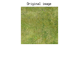
Compute the normalized kernel associated to u

[M,N,C] = size(u);
mu = repmat(mean(mean(u),2),[M N 1]);
tu = 1/sqrt(M*N)*(u-mu);

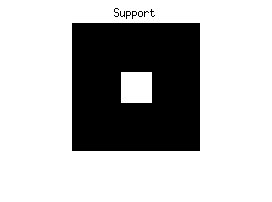
Definition of a rectangular support for the SOT

r = 15; % support half-size
M2 = floor(M/2)+1; N2 = floor(N/2)+1;
sup = zeros(M,N);
xind = M2-r:M2+r; m=2*r+1;
yind = N2-r:N2+r; n=2*r+1;
sup(xind,yind) = Inf;
suprgb = repmat(sup,[1 1 3]);
cardsup = sum(sum(sup>0));

figure
imshow(sup>0)
title('Support')

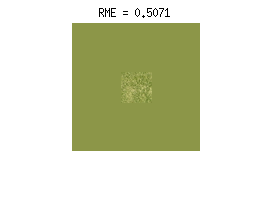
SOT computation

options.err = 1e-3;
options.nmax = 1000;
options.visu = 1;
options.nonverbose = 1;
t = so_texton(u,suprgb,options);

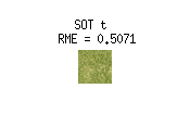
Crop the central part

tc = t(xind,yind,:);

muc = mu(xind,yind,:);

figure
imshow(muc+sqrt(m*n)*tc)
title(sprintf(['SOT t \n RME = ' ...
    num2str(otdist(tu,tc,M,N,1))]))

DSN synthesis

% Size of synthesis domain
Ms = 256;
Ns = 256;
nimp = 30; 
% number of impacts per pixel

% Mean image
mus = repmat(mu(1,1,:),[Ms Ns 1]);
% DSN
[sn,pp] = dsn(tc,mus,nimp/cardsup);
% ADSN (Gaussian limit)
adsnt = adsn(tc,mus);

figure
imshow(u)
title('Original texture u')
figure
imshow(adsnt)
title('ADSN(t)')
figure
imshow(sn)
title(['SN(t), ' num2str(nimp) ' impacts/pix'])

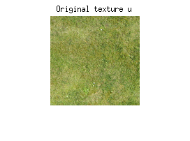
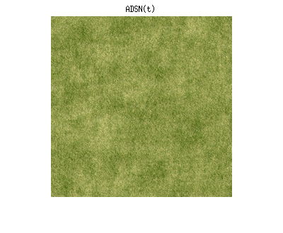
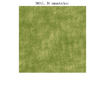
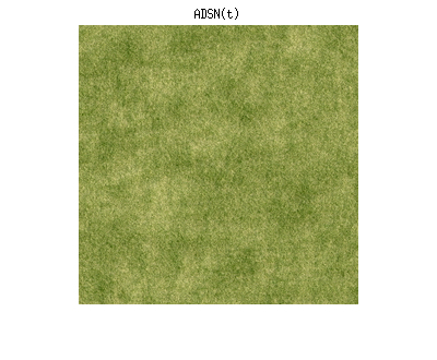
One can observe that SN(t) is a visually satisfying approximation of the Gaussian random field ADSN(t), even if the number of impacts per pixel is reasonably low.

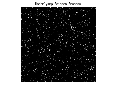
The underlying Poisson process is indeed sparse

figure
imshow(pp)
title('Underlying Poisson Process')

Comparison between the ADSN models

% ADSN associated to u
adsnu = adsn(tu,mus);

% Compute the Gaussian relative model error
gme = otdist(tu,t,Ms,Ns,1);

figure
imshow(adsnu)
title('ADSN(t_u)')
figure
imshow(adsnt)
title(['ADSN(t), RME = ' num2str(gme)])

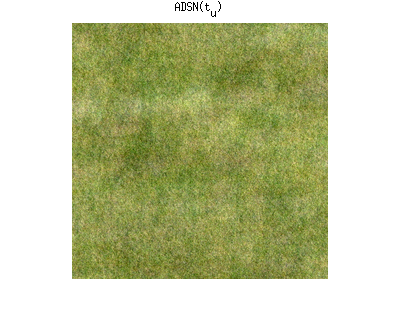
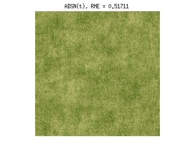
One can observe a slight loss in the color diversity when comparing u with SN(t), or when comparing ADSN(t_u) with ADSN(t). Indeed, the computation of the SOT does not ensure that the marginal color covariance of ADSN(t) is the same than the empirical color covariance of u. This will be confirmed by the next paragraph.

Color covariance

% Compute the matricial autocorrelation of t, which is the
%   marginal color covariance of ADSN(t)
act = zeros(C);
for i=1:C
    for j=1:C
        act(i,j) = sum(sum(t(:,:,i).*t(:,:,j)));
    end
end

% Empirical color covariance of u :
cov(reshape(u,[M*N 3]))
% Marginal color covariance of ADSN(t) :
act
% Empirical color covariance of adsnt :
cov(reshape(adsnt,[Ms*Ns 3]))

ans =

    0.0060    0.0047    0.0048
    0.0047    0.0045    0.0040
    0.0048    0.0040    0.0050


act =

    0.0047    0.0039    0.0041
    0.0039    0.0033    0.0034
    0.0041    0.0034    0.0036


ans =

    0.0046    0.0038    0.0040
    0.0038    0.0032    0.0033
    0.0040    0.0033    0.0035

Color covariance correction

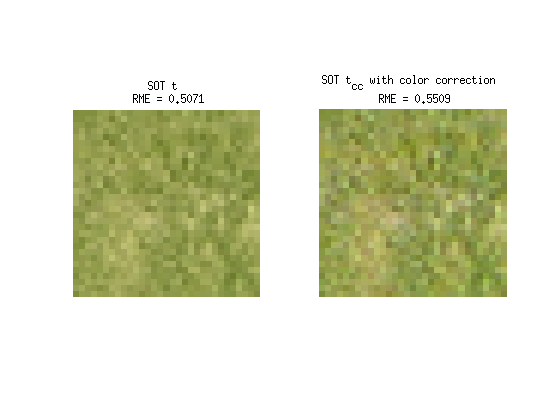
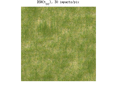
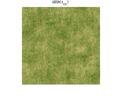
One can correct this color loss by applying a transformation in the color space so that the marginal color covariance of ADSN(t) matches the empirical color covariance of u.

tc_cc = cov_correction(tc,u);

% Visual comparison of the textons
muc = mu(xind,yind,:);
figure
subplot(1,2,1)
imshow(muc+sqrt(m*n)*tc)
title(sprintf(['SOT t \n RME = ' ...
    num2str(otdist(tu,tc,M,N,1))]))
subplot(1,2,2)
imshow(muc+sqrt(m*n)*tc_cc)
title(sprintf(['SOT t_{cc} with color correction \n RME = ' ...
    num2str(otdist(tu,tc_cc,M,N,1))]))

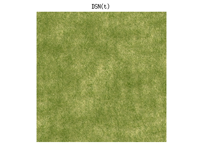
Comparison of the DSN synthesis results

sn_cc = dsn(tc_cc,mus,nimp/cardsup);

figure
imshow(sn)
title('DSN(t)')
figure
imshow(sn_cc)
title(['DSN(t_{cc}), ' num2str(nimp) ' impacts/pix'])

Comparison of the ADSN synthesis results

adsnt_cc = adsn(tc_cc,mus);

figure
imshow(adsnt)
title('ADSN(t)')
figure
imshow(adsnt_cc)
title('ADSN(t_{cc})')

The marginal color covariance is well corrected

act_cc = zeros(C);
for i=1:C
    for j=1:C
        act_cc(i,j) = sum(sum(tc_cc(:,:,i).*tc_cc(:,:,j)));
    end
end

% Empirical color covariance of u :
cov(reshape(u,[M*N 3]))
% Marginal color covariance of ADSN(t_{cc}) :
act_cc
% Empirical color covariance of adsnt_cc :
cov(reshape(adsnt_cc,[Ms*Ns 3]))

ans =

    0.0060    0.0047    0.0048
    0.0047    0.0045    0.0040
    0.0048    0.0040    0.0050


act_cc =

    0.0060    0.0047    0.0048
    0.0047    0.0045    0.0040
    0.0048    0.0040    0.0050


ans =

    0.0060    0.0048    0.0048
    0.0048    0.0045    0.0040
    0.0048    0.0040    0.0050

Tutorial on the Synthesis-Oriented Texton