Prévision d'un processus ARIMA

On considère le processus ARIMA(1,1,1) défini par

$$(1-\frac23B)(1-B) X_t = c + \varepsilon _t + \frac56 \varep... ... \mbox{o\\lq u}  \varepsilon \sim N(0,0.2^2) \mbox{et}  c=0.1;$$

1. Simuler, identifier et estimer les paramètre par methode de maximum de vraisemblance ($T=100$).

   Corrigé très peu de chagement par rapport à 3.2.4

    
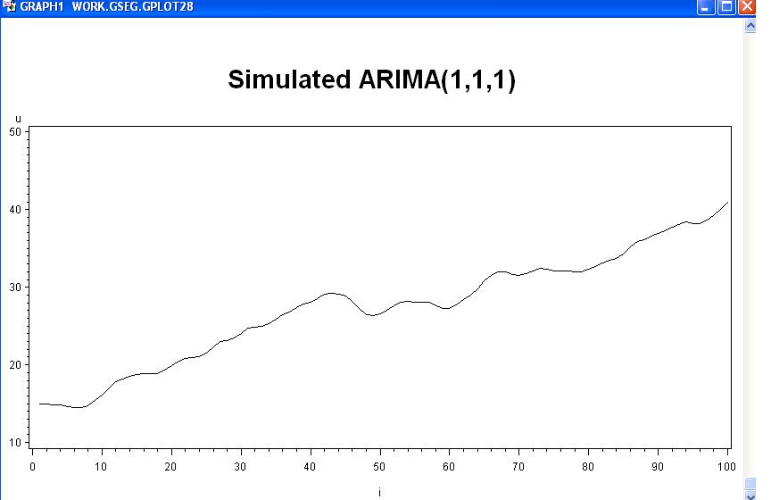
   title1 'Simulated ARIMA(1,1,1)';
   data a;
       u1=0; u2=0 ; a1 = 0;
       do i = -50 to 100;
          a = 0.2*rannor(1);
          u = 0.1 + (5.0/3)*u1 - (2.0/3)*u2 + a + (5.0/6)*a1;
          if i > 0 then output;         u2 = u1; u1 = u; a1 = a;
       end;
     run;
   
   symbol1 interpol=join color=black value=none;
   proc gplot data=a;
      plot u*i;
   run;
   title1 'arima (1,1,1)';
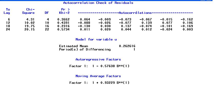
   proc arima data=a;
      identify var=u;run;
      identify var=u(1); run;
      estimate p=1 q=1 METHOD=ML; run;
   quit;
   

   
   
   Interprétation: D'apres le graphique, on constate que $X_t$ n'est pas stationnaire. SAS propose donc un modele ARIMA(1,1,1) avec constante
   
   $$\bgroup\color{blue} (1-0.57638B)X_t = c + (1+0.93229B)\varepsilon _t \egroup$$
   
   
   L'estimation pour $c=0.111249$. Le vrai modele est
   
   $$\bgroup\color{blue} (1-2/3B)X_t = 0.1 + (1+5/6B)\varepsilon _t \egroup$$
   
   
   Si on travaille avec nombre d'observation $T=1000$, on aura un meilleur résultat :
   
   $$\bgroup\color{blue} (1-0.57443B)X_t = c + (1+0.85768B)\varepsilon _t,   c = 0.1235 \egroup$$
   
   

2. Prévision à l'horizon $h=1,2,\cdots,20$.

   Corrigé une ligne à ajouter dans le procedure arima

    
   title1 'Simulated ARIMA(1,1,1)';
   data a;
       u1=0; u2=0 ; a1 = 0;
       do i = -50 to 100;
          a = 0.2*rannor(1);
          u = 0.1 + (5.0/3)*u1 - (2.0/3)*u2 + a + (5.0/6)*a1;
          if i > 0 then output;         u2 = u1; u1 = u; a1 = a;
       end;
     run;
   
   symbol1 interpol=join color=black value=none;
   proc gplot data=a;
      plot u*i;
   run;
   title1 'arima (1,1,1)';
   
   proc arima data=a;
      identify var=u;run;
      identify var=u(1); run;
      estimate p=1 q=1 METHOD=ML; run;
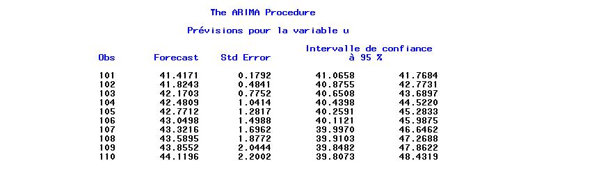
      forecast id=i lead=20 out=arima_1_1_1; run;
   quit;
   

   Les resultats sont stockés dans la base de donnée arima_1_1_1, prets à être exploités.
   
3. Tracer dans la même figure les observations, la prevision, et les intervalles de confiance de 95%.

   Corrigé On utilise la procedure gplot.

    
   \begin{verbatim} 
   title1 'Simulated ARIMA(1,1,1)';
   data a;
       u1=0; u2=0 ; a1 = 0;
       do i = -50 to 200; /* ici avec 100, l'estimation ne converge pas 
          a = 0.2*rannor(1);
          u = 0.1 + (5.0/3)*u1 - (2.0/3)*u2 + a + (5.0/6)*a1;
          if i > 0 then output;         u2 = u1; u1 = u; a1 = a;
       end;
     run;
   
   proc arima data=a;
      identify var=u;run;
      identify var=u(1); run;
      estimate p=1 q=1; run;
      forecast id=i lead=20 out=arima_1_1_1; run;
   quit;
   
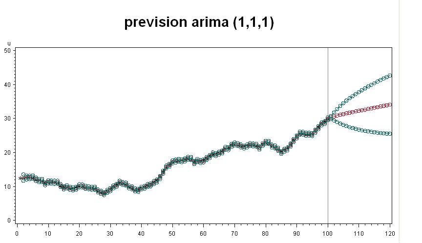
   title1 'prevision arima (1,1,1)';
   proc gplot data=arima_1_1_1;
      symbol1 i=join v=star h=1 cv=black ci=black co=black w=1;
      symbol2 i=join v=none h=3 cv=green ci=green co=green w=2;   
      symbol3 i=join v=none h=3 cv=red  ci=red   co=red   w=2; 
      plot u*i=1 forecast*i=2 (l95 u95)*i=3 /overlay href=100;
   run;
   quit;
   

   
4. Quels sont valeurs des paramètres que le procedure arima a estimés ?

   Corrigé

   
   
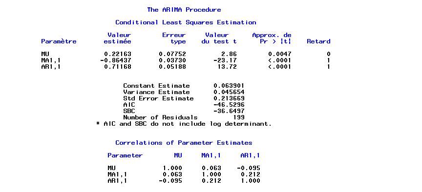
   Pour ce modèle, il y a 4 paramètres à estimer, en prenant rannor(2) et i=-50 to 200, nous avons

   	vrai valeur	Estimation
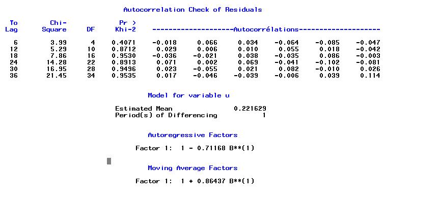
   AR(1)	$1-\frac23 B$	1 - 0.711 B**(1)
   MA(1)	$1+\frac56 B$	1 + 0.864 B**(1)
   c	0.1	0.0639
   $\sigma$	0.2	0.2136

   La taille $T=200$ d'observation ne nous permet pas d'obtenir une tres bonne estimation.
5. Pour obtenir une meilleures précision des estimations, on peut augumenter la taille $T$ à 10000. Re faire le calcul précédent.

   Corrigé En prenant rannor(2) et i=-50 to 10000,

   	vrai valeur	Estimation
   AR(1)	$1-\frac23 B$	1 - 0.6767 B**(1)
   MA(1)	$1+\frac56 B$	1 + 0.8292 B**(1)
   c	0.1	0.0926
   $\sigma$	0.2	0.200

   On note ces estimations sont assez proche des vraies valeurs
6. Refaire les previsions avec $T=1000$ avec $h=1,2,\cdots,40$. Mais cette fois tracer les observations apartir de 950 seulement.

   Corrigé Il y a pas grande chose à modifier par rapport a 3.3.3. Il faut ajouter quelques options à la fonction plot.

    
   title1 'prevision arima (1,1,1)';
   proc gplot data=arima_1_1_1;
      symbol1 i=join v=star h=1 cv=black ci=black co=black w=1;
      symbol2 i=join v=none h=3 cv=green ci=green co=green w=2;   
      symbol3 i=join v=none h=3 cv=red  ci=red   co=red   w=2; 
      plot u*i=1 forecast*i=2 (l95 u95)*i=3 /overlay
   	   haxis = 950 to 1040 href = 1000;
   run;
   quit;