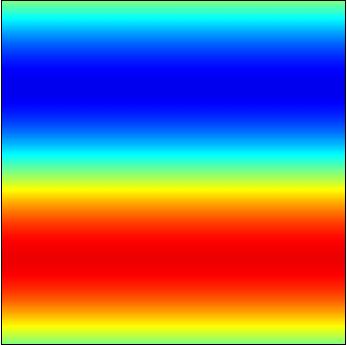
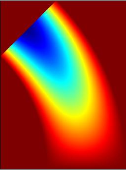
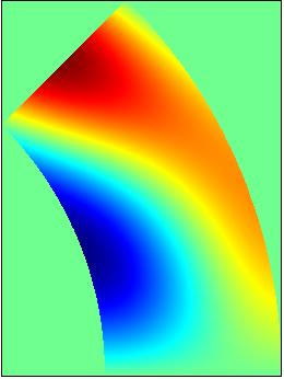
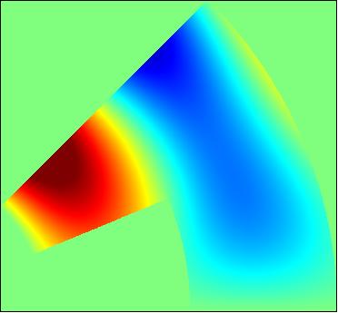
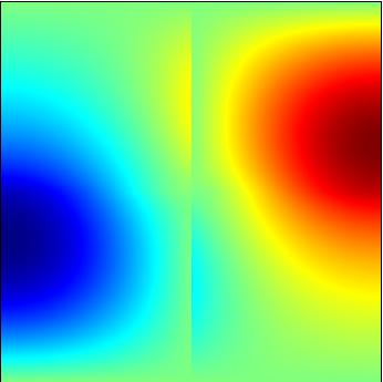
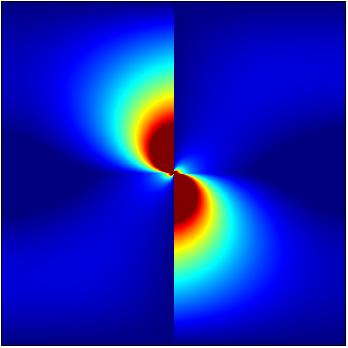
Benchmark computations for Maxwell equations
for the approximation of highly singular solutions.
Results from Inria Rocquencourt, computed with Montjoie
![]()
![]()
The benchmark problems are presented in the page BENCHMAX.
Authors, affiliation
Authors
Gary COHEN, Marc DURUFLE (numerical methods and computations)
Affiliation
Inria Rocquencourt (projet POEMS)
Coordinates
e-mail Marc.Durufle@inria.fr
web https://www.math.u-bordeaux.fr/~durufle
Method and code
The computations are done on isoparametric quadrilateral/hexahedral elements of Nedelec's first family.
To find the eigenvalues and eigenvectors, ARPACK library is used. As a shift-invert mode (cayley mode more precisely) is used, we have to solve several times a large linear system. We assume in these experiences that all the linear systems are solved directly by MUMPS.
Reference 1 :
Marc DURUFLE,
"Numerical integration and high order finite element methods
applied to time-harmonic Maxwell equations",2006
Phd Thesis in University Paris Dauphine.
Code Montjoie :
Marc DURUFLE.
Technical data:
Computations in double precision on a PC/Linux (3.2 Ghz, 2 Go of memory)
Results
Eigenvalues
|
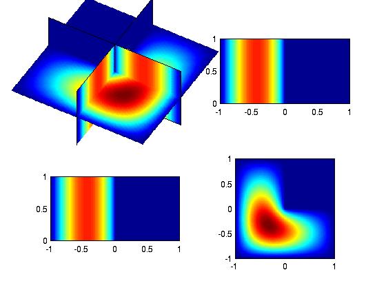
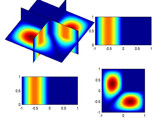
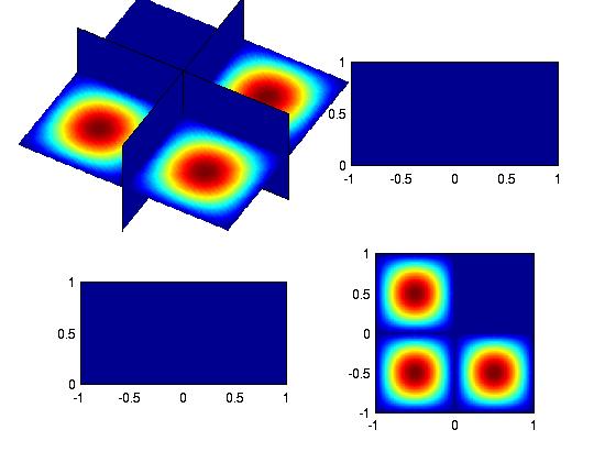
Maxwell eigenvalues in 2DomA (L-shape)
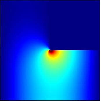
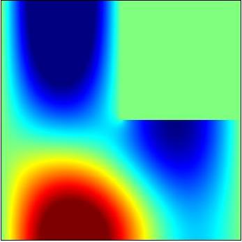
The reference eigenvalues are computed by nodal elements on a mesh locally refined near the vertex, with a high order of approximation (Q7). There are 59 459 degrees of freedom. The digits of all eigenvalues don't change, when we use a Q8 approximation.
|
1.47562182397e+00 3.53403136678e+00 9.86960440109e+00 9.86960440109e+00 1.13894793979e+01 |
It seems that these reference eigenvalues are equal to Monique Dauge''s eigenvalues, except for the first one (only 1 digit differs).
Let us see the errors when regular meshes are used, and NO local refinement is used.
| Q1, 10250 DOF | Q2, 10752 DOF | Q4, 9760 DOF | Q6, 10752 DOF | Q8, 9760 DOF |
|---|---|---|---|---|
|
1.74e-03 1.36e-04 4.89e-04 4.89e-04 4.31e-04 |
5.44e-04 1.26e-06 3.48e-07 3.48e-07 8.43e-07 |
2.28e-04 1.63e-07 < 1e-12 < 1e-12 7.28e-08 |
1.50e-04 6.81e-08 < 1e-12 < 1e-12 3.03e-08 |
1.13e-04 3.81e-08 < 1e-12 < 1e-12 1.69e-08 |
Now, the computations are done on regular meshes, and the lengths of the intervals follow a geometric progression, in order to have a local refinement near the singular vertex
| Q2, 10752 DOF | Q4, 9760 DOF | Q6, 10752 DOF | Q8, 9760 DOF | Q10, 9760 DOF |
|---|---|---|---|---|
|
5.40e-05 1.52e-06 6.17e-06 6.17e-06 5.43e-06 |
9.45e-07 5.00e-09 3.76e-08 3.76e-08 4.08e-08 |
5.00e-08 5.03e-10 3.89e-09 3.89e-09 3.78e-09 |
4.47e-08 3.39e-10 2.71e-12 2.71e-12 1.72e-10 |
4.95e-08 1.88e-10 < 1e-12 < 1e-12 7.74e-11 |
Now, the computations are done on triangular meshes, split in quadrilaterals. The advantage to use triangular meshes is to be able to locally refine near the vertex (without refining other parts of the domain). The main problem on this technique is the large amount of DOFS generated, because each triangle is split in three quadrilaterals.
| Q2, 10788 DOF | Q4, 9904 DOF | Q6, 10476 DOF |
|---|---|---|
|
6.59e-06 3.17e-07 5.69e-07 4.32e-07 6.60e-07 |
1.20e-06 3.07e-10 2.45e-07 1.82e-08 1.80e-07 |
9.02e-06 1.35e-08 < 1e-12 < 1e-12 5.77e-09 |
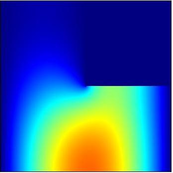
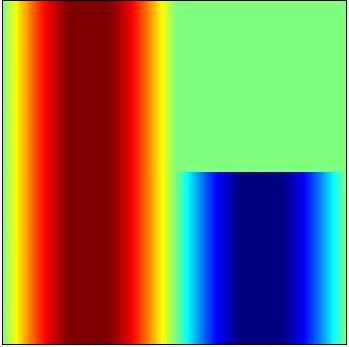
Maxwell eigenvalues in 2DomB (Cracked domain)
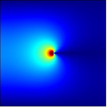
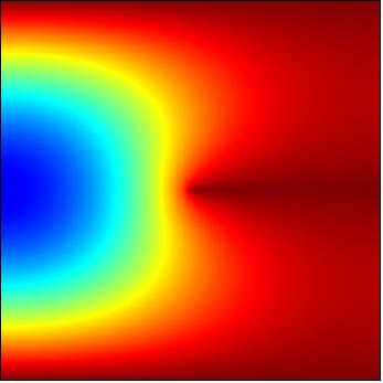
The reference eigenvalues are computed on a mesh locally refined near the vertex (0,0). Nodal elements are used, with a Neumann condition on the boundaries of the domain. The vertices of the crack are doubled, so that the scalar field can be discontinuous across the crack. For a Q6 approximation, the used mesh contains 127 525 degrees of freedom. All the digits of these eigenvalues don't change when the order of approximation is increased (Q7).
|
1.03407396876e+00 2.46740110027e+00 4.04692529140e+00 9.86960440109e+00 1.08448542781e+01 |
These eigenvalues are equal to those computed by Melina, except the first eigenvalue (the four last digits differ).
Let us see the errors when regular meshes are used, and NO local refinement is used.
| Q1, 20200 DOF | Q2, 20200 DOF | Q4, 21840 DOF | Q6, 18624 DOF | Q8, 18624 DOF |
|---|---|---|---|---|
|
9.10e-03 8.22e-05 9.38e-05 3.29e-04 3.29e-04 |
4.50e-03 1.08e-08 3.18e-07 1.73e-07 1.73e-07 |
2.39e-03 < 1e-12 2.74e-08 < 1e-12 < 1e-12 |
1.81e-03 < 1e-12 1.11e-08 < 1e-12 < 1e-12 |
1.34e-03 < 1e-12 < 1e-12 4.97e-09 < 1e-12 |
Now, the computations are done on the same regular meshes than previous, but the lengths of the intervals follow a geometric progression, in order to have a local refinement near the singular vertex
| Q2, 20200 DOF | Q4, 21840 DOF | Q6, 18624 DOF | Q8, 18624 DOF | Q10, 20200 DOF |
|---|---|---|---|---|
|
6.82e-05 8.78e-06 1.13e-05 4.59e-05 4.18e-05 |
1.51e-06 7.40e-09 1.37e-08 8.66e-07 8.66e-07 |
5.29e-07 1.59e-10 1.78e-09 1.10e-08 1.18e-08 |
4.53e-07 2.62e-10 8.84e-12 3.50e-12 5.64e-12 |
3.95e-07 2.02e-10 1.83e-09 < 1e-12 < 1e-12 |
Now, the computations are done on triangular meshes, split in quadrilaterals, with a local refinement.
| Q2, 20404 DOF | Q4, 21600 DOF | Q6, 20364 DOF |
|---|---|---|
|
7.16e-06 2.35e-08 2.96e-07 1.92e-06 6.82e-07 |
2.07e-06 < 1e-12 9.18e-10 1.28e-10 6.33e-10 |
2.53e-05 < 1e-12 4.94e-9 < 1e-12 < 1e-12 |
Maxwell eigenvalues in 2DomC (Part of a ring)
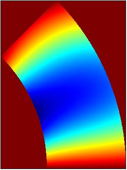
We obtain exactly the same reference eigenvalues than those computed by M. Dauge. We don't remind them. For the computations, isoparametric curved elements are used. This case is perfect for high order approximation.
| Q1, 202 DOF | Q2, 212 DOF | Q4, 212 DOF | Q7, 217 DOF | Q10, 220 DOF |
|---|---|---|---|---|
|
4.01e-03 1.58e-02 1.69e-02 1.50e-02 3.55e-02 |
9.51e-05 8.51e-04 2.66e-04 2.68e-04 4.01e-03 |
9.73e-08 4.36e-06 3.91e-07 6.19e-07 7.21e-04 |
3.98e-11 2.34e-09 3.58e-09 4.10e-09 6.78e-08 |
< 1e-12 1.15e-09 < 1e-12 < 1e-12 2.30e-06 |
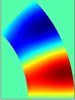
Maxwell eigenvalues in 2DomD (curved L-shape)
The reference eigenvalues are computed as usual on a mesh locally refined and with an order of approximation Q6. The used mesh contains 92 845 degrees of freedom. All the digits of these eigenvalues don't change when the order is increased (Q7)
|
1.81857115216e+00 3.49057623279e+00 1.06560150038e+01 1.01118862307+01 1.24355372481e+01 |
Let us see the errors when regular meshes are used, and NO local refinement is used.
| Q1, 10250 DOF | Q2, 10752 DOF | Q4, 9760 DOF | Q6, 10752 DOF | Q8, 9760 DOF |
|---|---|---|---|---|
|
1.83e-03 9.64e-05 4.97e-04 3.85e-04 9.19e-04 |
5.67e-04 3.65e-06 3.78e-07 9.25e-06 1.56e-04 |
2.71e-04 1.32e-6 1.18e-08 4.19e-6 7.44e-5 |
1.58e-04 6.98e-07 6.86e-09 2.42e-06 4.33e-05 |
1.19e-04 5.09e-07 5.19e-09 1.83e-06 3.28e-05 |
Now, the computations are done on the same regular meshes than previous, but the lengths of the intervals follow a geometric progression, in order to have a local refinement near the singular vertex
| Q2, 10250 DOF | Q4, 10752 DOF | Q6, 9760 DOF | Q8, 10752 DOF | Q10, 9760 DOF |
|---|---|---|---|---|
|
2.36e-05 3.14e-06 1.54e-05 1.23e-05 5.08e-05 |
1.06e-05 3.91e-08 1.89e-08 1.43e-07 2.92e-06 |
4.64e-06 1.70e-08 1.11e-10 6.97e-08 1.28e-06 |
3.92e-06 1.44e-08 1.04e-10 5.89e-08 1.08e-06 |
3.02e-06 1.10e-08 8.14e-11 4.53e-08 8.32e-07 |
Now, the computations are done on triangular meshes, split in quadrilaterals, with a local refinement.
| Q2, 10814 DOF | Q4, 10272 DOF | Q7, 12460 DOF |
|---|---|---|
|
3.28e-06 3.77e-07 1.21e-06 8.76e-07 1.66e-06 |
8.03e-07 6.23e-09 1.64e-10 1.19e-08 2.27e-07 |
6.70e-07 5.32e-09 3.04e-11 1.08e-08 1.82e-07 |
Maxwell eigenvalues for piecewise constant permittivity in 2DomE (Square)
The reference eigenvalues are computed with nodal finite elements on a mesh locally refined with a high order approximation (Q7). Only 11 digits don't change when the order of approximation is increased (Q8). For a Q8 approximation, the mesh contains 629 953 degrees of freedom. The 12th digit can be false.
|
\epsilon_1 = 0.10 \nu = 0.38996445808427 |
0.4533851871670E+01 0.6250319385542E+01 0.7037074196013E+01 0.2234193733539E+02 0.2267919225110E+02 0.2609520278068E+02 0.2650900637498E+02 0.4048783516243E+02 0.4265069898070E+02 0.5588227467094E+02 |
|
\epsilon_1 = 0.01 \nu = 0.12690206972221 |
0.4893193324883E+01 0.7206675422497E+01 0.1526169708758E+02 0.2446225024727E+02 0.2448745601340E+02 0.2775724058215E+02 0.2949978412416E+02 0.4424890377211E+02 0.4443521693426E+02 0.6359570343398E+02 |
For this case, we don't provide computations with the first family of Nedelec, because Arpack suffer from problems when generalized eigenvalue problems have to be solved, and when the mesh presents a very high ratio between the largest element and the the smallest element. We didn't observe this problem for the solution of standard real symmetric eigenvalue problems.
Maxwell eigenvalues in 3DomA (Thick L-shape)

We consider the reference eigenvalues given by M. Dauge. Let us see the eigenvalues and the errors when regular meshes are used, with a local refinement. The 3-D mesh is generated by extrusion of a 2-D mesh of the L-shaped geometry. In the direction of extrusion, there is a few layers (by exemple one layer for Q8). We compare different orders of approximation with almost the same number of dofs (about 120 000).
| Q2, 115 224 DOF | Q4, 127 528 DOF | Q5, 120 550 DOF | Q8, 127 528 DOF | Q9, 115 497 DOF |
|---|---|---|---|---|
|
9.6405320333e+00 1.1342449138e+01 1.3400983075e+01 1.5197331684e+01 1.9507478040e+01 1.9736612931e+01 |
9.6397331487e+00 1.1345221291e+01 1.3403632246e+01 1.5197246134e+01 1.9509334010e+01 1.9739204891e+01 |
9.6397258597e+00 1.1345225905e+01 1.3403635730e+01 1.5197261357e+01 1.9509330243e+01 1.9739207757e+01 |
9.6397242598e+00 1.1345226159e+01 1.3403635766e+01 1.5197251939e+01 1.9509328660e+01 1.9739208800e+01 |
9.6397247956e+00 1.1345226075e+01 1.3403635766e+01 1.5197251946e+01 1.9509329197e+01 1.9739208800e+01 |
| Q2, 115 224 DOF | Q4, 127 528 DOF | Q5, 120 550 DOF | Q8, 127 528 DOF | Q9, 115 497 DOF |
|---|---|---|---|---|
|
8.39e-05 2.45e-04 1.98e-04 5.25e-06 9.48e-05 1.32e-04 |
9.65e-07 4.34e-07 2.63e-07 3.81e-07 2.95e-07 1.98e-07 |
2.09e-07 2.82e-08 2.80e-09 6.21e-07 1.02e-07 1.00e-07 |
4.31e-08 5.86e-09 1.44e-10 8.55e-10 2.12e-08 1.23e-10 |
9.86e-08 1.32e-08 1.49e-10 1.29e-09 4.87e-08 1.13e-10 |
Maxwell eigenvalues in 3DomB (Fichera corner)
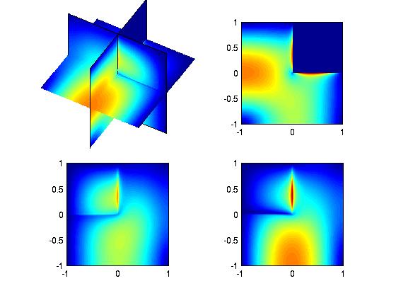
We don't have any reference eigenvalues for this case. We are not able to have a good accuracy with our code. Our finest mesh contains 177 720 dofs (for a Q5 approximation). we can estimate the accuracy of the computed eigenvalues as following :
| Eigenvalues | Number of hopefully reliable digits | Guess for the next digit - conjectured eigenvalue |
|---|---|---|
|
3.21987401386e+00 5.88041891178e+00 5.88041891780e+00 1.06854921311e+01 1.06937829409e+01 1.06937829737e+01 1.23165204656e+01 1.23165204669e+01 |
4 6 6 4 5 5 6 6 |
3.2199???e+00 5.88041??e+00 5.88041??e+00 1.06854??e+01 1.06937??e+01 1.06937??e+01 1.23164??e+01 1.23164??e+01 |
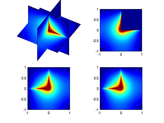
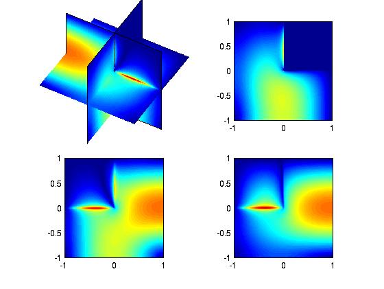
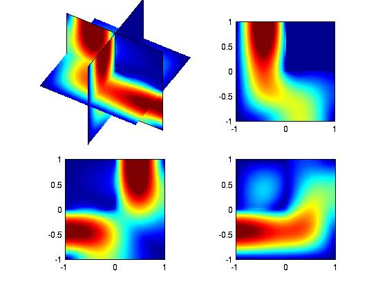
The first eigenvalue is simple and the corresponding eigenvector has the most singular part possible (the Fichera exponent is visible at the corner).
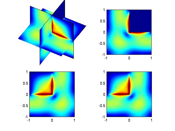
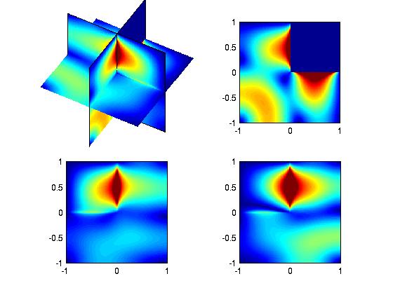
The eigenvalues 2 and 3 are double. The eigenvalue 4 has a non-smooth eigenvector and is single.
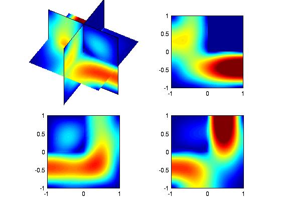
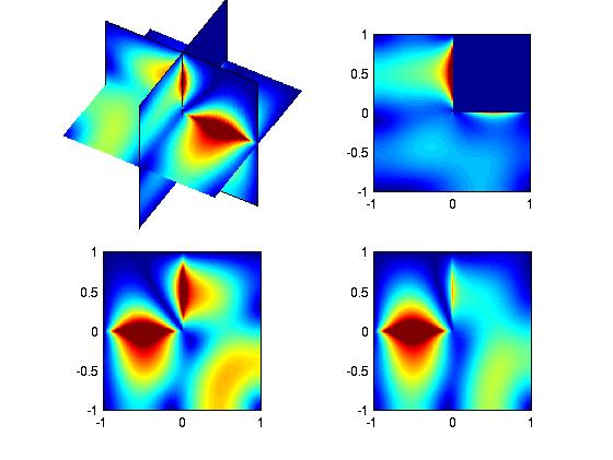
The eigenvalues 5 and 6 are double and the corresponding eigenvectors are "smooth" .
The eigenvalues 7 and 8 are double. If we consider these eigenvalues as reference, one has the following results
| Q2, 39 816 DOF | Q4, 39 816 DOF | Q6, 39 816 DOF | Q8, 127 528 DOF |
|---|---|---|---|
|
3.2123993016e+00 5.8809607342e+00 5.8809607404e+00 1.0692793589e+01 1.0705306226e+01 1.0705306231e+01 1.2314537441e+01 1.2314537464e+01 |
3.2193889658e+00 5.8804503696e+00 5.8804503880e+00 1.0685765274e+01 1.0694406173e+01 1.0694406213e+01 1.2315771855e+01 1.2315771918e+01 |
3.2195434724e+00 5.8804399916e+00 5.8804400049e+00 1.0685819390e+01 1.0694300944e+01 1.0694300980e+01 1.2316410983e+01 1.2316411024e+01 |
3.2197845160e+00 5.8804250009e+00 5.8804250019e+00 1.0685576624e+01 1.0693921375e+01 1.0693921377e+01 1.2316474407e+01 1.2316474410e+01 |
| Q2, 39 816 DOF | Q4, 39 816 DOF | Q6, 39 816 DOF | Q8, 92 256 DOF |
|---|---|---|---|
|
2.32e-03 9.21e-05 9.21e-05 6.83e-04 1.08e-03 1.08e-03 1.61e-04 1.61e-04 |
1.51e-04 5.35e-06 5.35e-06 2.56e-05 5.83e-05 5.83e-05 6.08e-05 6.08e-05 |
1.03e-04 3.58e-06 3.59e-06 3.06e-05 4.84e-05 4.84e-05 8.89e-06 8.89e-06 |
2.78e-05 1.04e-06 1.03e-06 7.91e-06 1.30e-05 1.30e-05 3.74e-06 3.74e-06 |