Research

Truly multi-dimensional numerical methods
While physical diffusion (i.e. in the Navier-Stokes equations) is imposed by modeling, numerical diffusion serves the only purpose of stabilizing the method, and should be otherwise as invisible as possible. In multi-d, simple choices of numerical diffusion are not satisfactory.
Let me exemplify this on the concept of stationarity preservation. In multi-d, stationary states of a system of conservation laws are such that the x-derivative of the x-flux, the y-derivative of the y-flux etc, all summed up, vanish. In particular, these derivatives do not in general vanish individually, and the stationary state is not a uniform constant (think of a vortex for the Euler eqautions, for example).
Consider now a numerical method for the instationary problem that adds numerical diffusion in all variables (e.g. a simple Laplacian). Of course, if it is fed initial data that are solutions of the stationary equation, one would wish the numerical solution to not evolve much (this is the rough idea behind stationarity preservation, see here for a precise definition). However, the long term solution of the heat equation (e.g. on a periodic domain) is a uniform constant. Adding a Laplacian in all variables will essentially drive the initial data towards uniform constants. In other words, the (non-constant) initial datum that one expected to remain (approximately) stationary is instead decaying exponentially quickly. Grid refinement changes the speed of decay, but not the qualitative picture.
The idea behind stationarity preserving methods is to choose a better numerical diffusion, that does not act on stationary states (i.e. it has a large kernel). One example is grad div. If the stationary states of the PDE are given by a divergence-free vector field (as is the case for linear acoustics), then such a diffusion operator will ignore them. Of course, one needs to guarantee that instationary problems are still evolved in a stable way, and this balance makes the choice of the right diffusion and the quest for guiding principles challenging.
Active Flux
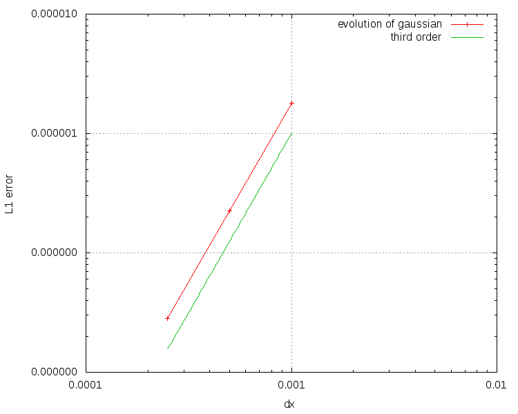
The Active Flux scheme is a recent extension of the finite volume scheme. It uses additional pointwise degrees of freedom, continuous reconstructions and is third order accurate. You can find more details here:
Active Flux on arXiv
Barsukow, Hohm, Klingenberg, Roe 2018,
Eymann, Roe 2011,
van Leer 1977
If you are interested to try out the Active Flux scheme you can find here a tiny code that implements Active Flux for linear advection in 1d: miniActiveFlux (bitbucket.org). NEW: A limiting strategy (see below) is now part of the tiny code!
Some snapshots (produced with the above minimal code):
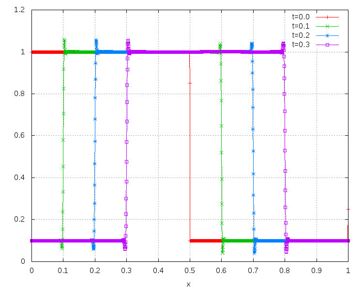
There is a limiting strategy for Active Flux explained in Barsukow, 2021. This limiting does not remove all extrema, but it improves the solution significantly. Here is an example of the behaviour of the limited solution for large CFL numbers:
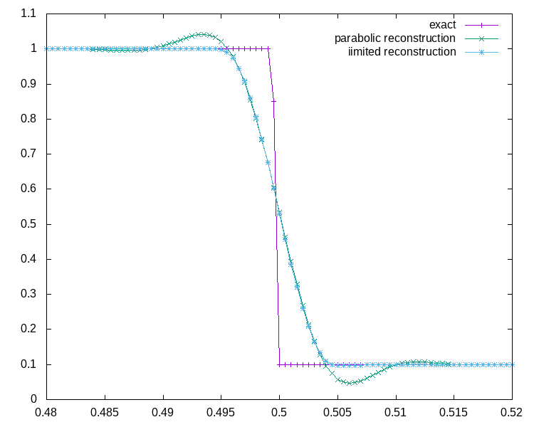
You can play with the limited reconstruction in this interactive plot. Move the two point values and the average, and observe how the parabola (dashed) is replaced by power laws whenever the parabola has an artificially non-monotone behaviour.
More sophisticated implementations allow to compute following examples:
Shallow water equations with wetting and drying
Kelvin-Helmholtz instability
Delaunay-like multi-d Riemann Problems for isentropic Euler (see the Art and Science section for more background)


Right: For comparison results with Roe 1981.
Linear stability
For systems or high order methods, linear (von Neumann) stability analysis requires to check whether the eigenvalues of some complex-valued matrix are located inside the unit disc. It is unnecessary (and often very complicated) to compute these eigenvalues. There exist necessary and sufficient conditions for this (discovered by Schur in 1917/18) which do not involve computing the eigenvalues. The starting point is the characteristic polynomial of the matrix.
I have here some slides discussing the proof (following Miller 1971). In principle, you can perform the analysis analytically, but if your matrix/polynomial depends on parameters, the stability region in the parameter space might turn out to be very complicated. For this case, here is a tiny code (in Java) that implements the algorithm and allows for parameter studies. The important function is boolean isNeumann in class Miller.
Last modified: Wed Oct 02 09:26:04 CEST 2024