Univariate and multivariate polynomials
A basic implemententation is proposed for handling univariate and multivariate polynomials (represented by their coefficients). You should use those classes carefully for two reasons :
- The implementation is not optimal for multivariate polynomials (loops are not unrolled as for tiny vectors). Maybe this drawback will be removed in future versions of Montjoie
- The use of Horner's algorithm may lead to instability when the order of polynomial becomes too large. For example, you should not use those classes for Legendre polynoms, but rather the functions GetJacobiPolynomial and EvaluateJacobiPolynomial, or the class LegendrePolynomial detailed below.
So these classes are useful for developing, testing new methods. Here we briefly describe how to use them.
Basic Use
First, we show examples for 1-D polynomials (univariate) :
// first we create two useful polynoms : 1 and x
UnivariatePolynomial<double> x(1), one(0);
x(0) = 0; x(1) = 1.0;
one(0) = 1.0;

// then you can construct other polynomials with those basic polynoms
// for example chebyshev polynomials are constructed  :
UnivariatePolynomial<double> Pn_m1, Pn, Pn_p1;
Pn_m1 = one;
Pn = x;
int n = 10;
for (int k = 1; k < n; k++)
  {
    Pn_p1 = 2.0*x*Pn - Pn_m1;
    Pn_m1 = Pn;
    Pn = Pn_p1;
  }

// of course you can enter directly coefficients
// P = a0 + a1 X + a2 X^2 + .. + an x^n
UnivariatePolynomial<double> P;
P.SetOrder(n);
P(0) = a0;
P(1) = a1;
// ...
P(n) = an;

// and evaluate y = P(x) for a given x with Horner algorithm :
double y = P.Evaluate(2.53);

// and operators -, +, * can be used
UnivariatePolynomial<double> Q, R, S;
S = 2.5*P*Q + R;

// polynoms can be derived or integrated (with 0-constant)
UnivariatePolynomial<double> dP_dx, Primitive_P;
DerivatePolynomial(P, dP_dx);
IntegratePolynomial(P, Primitive_P);
For multivariate polynomials, the degree of the polynom is the sum of the degree for each variable.
// for 3-D polynoms, we create 1, x, y and z
// the first argument of the constructor is the number of variables
// by default, we set all the coefficients to 0
MultivariatePolynomial<double> x(3, 1), one(3, 0), y(3, 1), z(3,
1);
one(0, 0, 0) = 1.0
x(1, 0, 0) = 1.0;
y(0, 1, 0) = 1.0;
z(0, 0, 1) = 1.0;

// then you can construct other polynomials with those basic polynoms
MultivariatePolynomial<double> P;
P = x*(x + 2.5*y*z);

// of course you can enter directly coefficients
P.SetOrder(3, n);
P(0, 0, 0) = a000;
P(1, 0, 0) = a100;
// ...
P(n, 0, 0) = an00;
P(0, n, 0) = a0n0;
P(0, 0, n) = a00n;

// and evaluate y = P(x) for a given x with Horner algorithm :
TinyVector<double, 3> pt(-3.4, 2.31, 0.56);
double value = P.Evaluate(pt);

// and operators -, +, * can be used
MultivariatePolynomial<double> Q, R, S;
S = 2.5*P*Q + R;

// polynoms can be derived or integrated (with 0-constant)
MultivariatePolynomial<double> dP_dx, dP_dy, Primitive_Px;
DerivatePolynomial(P, dP_dx, 0);
DerivatePolynomial(P, dP_dy, 1);
IntegratePolynomial(P, Primitive_Px, 0);

// operator () has been overloaded for 2-D and 3-D polynoms
// for higher dimensions, you have to use IndexToPowers, PowersToIndex
// for example in 4-D :
MultivariatePolynomial<double> t;
one.SetOrder(4, 1);
x.SetOrder(4, 1);
y.SetOrder(4, 1);
z.SetOrder(4, 1);
t.SetOrder(4, 1);

IVect powers(4);
powers.Fill(0);
int pos = one.PowersToIndex(powers);
one(pos) = 1.0;

powers(0) = 1;
pos = x.PowersToIndex(powers);
x(pos) = 1.0;

powers(0) = 0; powers(1) = 1;
pos = y.PowersToIndex(powers);
y(pos) = 1.0;

powers(1) = 0; powers(2) = 1;
pos = z.PowersToIndex(powers);
z(pos) = 1.0;

powers(2) = 0; powers(3) = 1;
pos = t.PowersToIndex(powers);
t(pos) = 1.0;
Methods for univariate polynomials
| constructors | |
| operators | |
| GetOrder | returns the degree of polynomial |
| SetOrder | modifies the degree of polynomial and removes previous coefficients |
| ResizeOrder | modifies the degree of polynomial and keeps previous coefficients |
| Zero | sets all coefficients to 0 |
| Evaluate | evaluates the polynomial with Horner algorithm |
Methods for the class LegendrePolynomial
| constructor | |
| EvaluateDerivative | evaluates Pn(cos θ) and its derivatives |
| EvaluatePn | evaluates Legendre polynomials at a given point |
| EvaluateDerive | evaluates Legendre polynomials and derivatives |
Methods for the class AssociatedLegendrePolynomial
| Init | inits the computation of associated Legendre polynomials |
| EvaluatePnm | evaluates associated Legendre polynomials |
Functions for univariate polynomials
| Pow | Computes a power of the polynomial |
| DerivatePolynomial | Computes the derivative of a polynomial |
| IntegratePolynomial | Computes the primitive of a polynomial |
| ComputeLegendrePolynome | Computes Legendre polynomials |
| Add | adds two polynomials |
| Mlt | computes the product of two polynomials |
| MltAdd | adds the product of two polynomals |
| SolvePolynomialEquation | finds the roots of a polynomial |
Methods for multivariate polynomials
| constructors | |
| operators | |
| GetM | returns the number of coefficients of the polynomial |
| GetDimension | returns the number of variables (called dimension) |
| GetOrder | returns the degree of polynomial |
| SetOrder | modifies the degree and dimension of polynomial and removes previous coefficients |
| ResizeOrder | modifies the degree and dimension of polynomial and keeps previous coefficients |
| Zero | sets all coefficients to 0 |
| Evaluate | evaluates the polynomial with Horner algorithm |
| PowersToIndex | computes scalar index from the tuple (i, j, ...) |
| IndexToPowers | computes the tuple (i, j, ...) from the scalar index |
| PrintRational | displays coefficients as fractions |
| PrintMonomial | displays a single monomial of the polynomial |
Functions for multivariate polynomials
| Pow | Computes a power of the polynomial |
| DerivatePolynomial | Computes the derivative of a polynomial |
| Derivate | Computes the derivative of a polynomial |
| GetCurlPolynomial | Computes the curl of a 3-D vector of polynomials |
| GetDivPolynomial | Computes the divergence of a 3-D vector of polynomials |
| IntegratePolynomial | Computes the primitive of a polynomial |
| Mlt | computes the product of a polynomial with a scalar |
| MltAdd | adds the product of two polynomals |
| IntegrateOnSimplex | computes the integral of the polynomial over the simplex (triangle in 2-D, tetrahedron in 3-D) |
| Add | adds two polynomials |
| ScalePolynomVariable | all the variables of the polynomial are multiplied by the same coefficient |
| CompressPolynom | sets to 0 small coefficients of the polynomial |
| OppositeX | x-variable is replaced by its opposite |
| OppositeY | y-variable is replaced by its opposite |
| PermuteXY | x-variable and y-variable are swapped |
| GenerateSymPol | generates polynomials obtained by symmetry with respect to diagonals of the square [-1, 1]2 |
| GenerateSym4_Edges | generates polynomials obtained by symmetry with respect to axis x=0 and y=0 of the square [-1, 1]2 |
| GenerateSym8 | generates polynomials obtained by symmetry with respect to diagonals and axis x=0 and y=0 of the square [-1, 1]2 |
Constructors for UnivariatePolynomial
Syntax
  UnivariatePolynomial();
  UnivariatePolynomial(int order);
The default constructor creates a polynomial equal to 0 (of degree 0). The second constructor takes the degree of the polynomial as argument and initializes all coefficients to 0.
Example :
// P is equal to 0
UnivariatePolynomial<Real_wp> P;

// P = 2x^2 + 5x - 8
UnivariatePolynomial<Real_wp> P(2);
P(0) = -8.0; P(1) = 5.0; P(2) = 2.0;
Location :
Share/UnivariatePolynomialInline.cxx
Operators for UnivariatePolynomial
The operators +, -, * are implemented for univariate polynomials and as well as operators +=, -= and *=. The operator * can mix scalars with polynomials.
Example :
// P is equal to 0
UnivariatePolynomial<Real_wp> P;

// P = 2x^2 + 5x - 8
UnivariatePolynomial<Real_wp> P(2), Q(3), R;
P(0) = -8.0; P(1) = 5.0; P(2) = 2.0;

// Q = x^3 - 7 x
Q(3) = 1.0; Q(1) = -7.0;

// R = 2.0 P Q - 3.0 P
R = 2.0*P*Q - 3.0*P;

// Q = Q + R
Q += R;
Location :
Share/UnivariatePolynomialInline.cxx
GetOrder
Syntax
int GetOrder() const;
This method returns the degree of the polynomial.
Example :
// P is equal to 0
UnivariatePolynomial<Real_wp> P;

// P = 2x^2 + 5x - 8
UnivariatePolynomial<Real_wp> P(2);
P(0) = -8.0; P(1) = 5.0; P(2) = 2.0;

// P.GetOrder() should return 2
int deg = P.GetOrder();
Location :
Share/UnivariatePolynomialInline.cxx
SetOrder
Syntax
void SetOrder(int k);
This method modifies the degree of the polynomial and sets all coefficients of the polynomial to 0.
Example :
// P is equal to 0
UnivariatePolynomial<Real_wp> P;

// P = 2x^2 + 5x - 8
UnivariatePolynomial<Real_wp> P(2);
P(0) = -8.0; P(1) = 5.0; P(2) = 2.0;

// we change the degree of P : all coefficients are set to 0
P.SetOrder(4);
P(0) = 2.5; P(2) = -4.1; P(4) = 6.0;
Location :
Share/UnivariatePolynomial.cxx
ResizeOrder
Syntax
void ResizeOrder(int k);
This method modifies the degree of the polynomial and sets new coefficients of the polynomial to 0. Old coefficients are kept.
Example :
// P is equal to 0
UnivariatePolynomial<Real_wp> P;

// P = 2x^2 + 5x - 8
UnivariatePolynomial<Real_wp> P(2);
P(0) = -8.0; P(1) = 5.0; P(2) = 2.0;

// we change the degree of P and we keep old coefficients
P.SetOrder(4);
// P = 4x^4 + 3 x^3 + 2x^2 + 5x - 8
P(4) = 4.0; P(3) = 3.0;
Location :
Share/UnivariatePolynomial.cxx
Zero
Syntax
void Zero();
This method sets all coefficients to 0.
Example :
// P is equal to 0
UnivariatePolynomial<Real_wp> P;

// P = 2x^2 + 5x - 8
UnivariatePolynomial<Real_wp> P(2);
P(0) = -8.0; P(1) = 5.0; P(2) = 2.0;

// P = 0
// P is not resized, coefficients are just set to 0
P.Zero();
Location :
Evaluate
Syntax
T Evaluate(T x);
This method evaluates the polynomial at a given point x with Horner's algorithm.
Example :
// P is equal to 0
UnivariatePolynomial<Real_wp> P;

// P = 2x^2 + 5x - 8
UnivariatePolynomial<Real_wp> P(2);
P(0) = -8.0; P(1) = 5.0; P(2) = 2.0;

// we compute y = P(x)
Real_wp x = 5.0;
Real_wp y = P.Evaluate(x);
Location :
Share/UnivariatePolynomial.cxx
Constructor for LegendrePolynomial
Syntax
LegendrePolynomial(int n);
The constructor takes the maximum number of Legendre polynomials to evaluate.
Example :
// coefficients of the recurrence are computed
int n = 10;
LegendrePolynomial<Real_wp> P(n);

// now we can evaluate P_0(x), P_1(x), ..., P_{n-1}(x)
// where P_k is the k-th Legendre polynomial
VectReal_wp EvalP;
Real_wp x = 0.4;
P.EvaluatePn(n, x, EvalP);
Location :
Share/UnivariatePolynomial.cxx
EvaluateDerivative
Syntax
void EvaluateDerivative(int n, T cos_teta, T sin_teta, Vector& Pn0, Vector& Pn1, Vector& dPn1);
This method evaluates Pn(cos θ) where Pn are Legendre polynomials. It also evaluates sin θ P'n(cos θ) and the derivative of this expression.
Example :
// coefficients of the recurrence are computed
int n = 10;
LegendrePolynomial<Real_wp> P(n);

// P_k(cos teta) are evaluated for k = 0..n-1
// P_k^1 = sin teta P'_k(cos teta) are also evaluated
// and the derivatives of P_k^1 = cos teta P'_k(cos_teta) - sin^2 teta P''_k(cos_teta)
// where P_k is the k-th Legendre polynomial
VectReal_wp EvalP, EvalP1, dP1;
Real_wp teta = pi_wp/4, cos_teta = cos(teta), sin_teta = sin(teta);
P.EvaluateDerivative(n, cos_teta, sin_teta, EvalP, EvalP1, dP1);
Location :
Share/UnivariatePolynomial.cxx
EvaluatePn
Syntax
void EvaluatePn(int n, T x, Vector& EvalP);
This method evaluates the Legendre polynomials P0, P1, ..., Pn-1 at a given point.
Example :
// coefficients of the recurrence are computed
int n = 10;
LegendrePolynomial<Real_wp> P(n);

// now we can evaluate P_0(x), P_1(x), ..., P_{n-1}(x)
// where P_k is the k-th Legendre polynomial
VectReal_wp EvalP;
Real_wp x = 0.4;
P.EvaluatePn(n, x, EvalP);
Location :
Share/UnivariatePolynomial.cxx
EvaluateDerive
Syntax
void EvaluateDerive(int n, T x, Vector& EvalP, Vector& dP);
This method evaluates the Legendre polynomials P0, P1, ..., Pn-1 at a given point and the derivatives.
Example :
// coefficients of the recurrence are computed
int n = 10;
LegendrePolynomial<Real_wp> P(n);

// now we can evaluate P_0(x), P_1(x), ..., P_{n-1}(x)
// where P_k is the k-th Legendre polynomial
// and the derivatives P'_0(x), P'_1(x), ..., P'_{n-1}(x)
VectReal_wp EvalP, derP;
Real_wp x = 0.4;
P.EvaluateDerive(n, x, EvalP, derP);
Location :
Share/UnivariatePolynomial.cxx
Init
Syntax
void Init(int Lmax)
This method comptes coefficients involved in reccurence relation used to evaluate normalized associated Legendre polynomials. They are defined as:

where
 are the usual associated Legendre polynomials satisfying the
recurrence:
are the usual associated Legendre polynomials satisfying the
recurrence:

The normalization
factor is designed such that the L2 norm of polynomials
 over the sphere is equal to one.
Example :
// coefficients of the recurrence are computed
// we need to know the maximal value of l
int Lmax = 100;
AssociatedLegendrePolynomial<Real_wp> P(Lmax);

// now we can evaluate \bar{P}_l^m(cos teta)
// these coefficients are stored in EvalP(l)(m)
// and computed for l = 0..Lmax
Vector<VectReal_wp> EvalP;
Real_wp teta = pi_wp/4;
P.EvaluatePnm(Lmax, Lmax, teta, EvalP);
Location :
Share/UnivariatePolynomial.cxx
EvaluatePnm
Syntax
void EvaluatePnm(int Lmax, int Mmax, T teta, Vector<Vector>& EvalP);
This methods evaluates normalized associated Legendre polynomials. They are defined as:
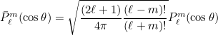
where
 are the usual associated Legendre polynomials satisfying the
recurrence:
are the usual associated Legendre polynomials satisfying the
recurrence:

The normalization
factor is designed such that the L2 norm of polynomials
 over the sphere is equal to one. The polynomials are evaluated for
l=0..Lmax and for m=0..min(l, Mmax).
over the sphere is equal to one. The polynomials are evaluated for
l=0..Lmax and for m=0..min(l, Mmax).
Example :
// coefficients of the recurrence are computed
// we need to know the maximal value of l
int Lmax = 100;
AssociatedLegendrePolynomial<Real_wp> P(Lmax);

// now we can evaluate \bar{P}_l^m(cos teta)
// these coefficients are stored in EvalP(l)(m)
// and computed for l = 0..Lmax
Vector<VectReal_wp> EvalP;
Real_wp teta = pi_wp/4;
// The second argument can be lower than Lmax, if you do not want to compute all polynomials m=0..l
P.EvaluatePnm(Lmax, Lmax, teta, EvalP);
Location :
Share/UnivariatePolynomial.cxx
Pow
Syntax
UnivariatePolynomial Pow(const UnivariatePolynomial& P, int n);
This functions returns the power of a polynomial.
Example :
// P is equal to 0
UnivariatePolynomial<Real_wp> P, Q;

// P = 2x^2 + 5x - 8
UnivariatePolynomial<Real_wp> P(2);
P(0) = -8.0; P(1) = 5.0; P(2) = 2.0;

// if you want to compute Q = P^4
Q = Pow(P, 4);
Location :
Share/UnivariatePolynomial.cxx
DerivatePolynomial
Syntax
void DerivatePolynomial(const UnivariatePolynomial& P, UnivariatePolynomial& Q);
This functions computes the derivative of a polynomial.
Example :
// P is equal to 0
UnivariatePolynomial<Real_wp> P, Q;

// P = 2x^2 + 5x - 8
UnivariatePolynomial<Real_wp> P(2);
P(0) = -8.0; P(1) = 5.0; P(2) = 2.0;

// if you want to compute Q = P' = 4x + 5 here
DerivatePolynomial(P, Q);
Location :
Share/UnivariatePolynomial.cxx
IntegratePolynomial
Syntax
void IntegratePolynomial(const UnivariatePolynomial& P, UnivariatePolynomial& Q);
This functions computes the primitive of a polynomial that cancels for x=0.
Example :
// P is equal to 0
UnivariatePolynomial<Real_wp> P, Q;

// P = 2x^2 + 5x - 8
UnivariatePolynomial<Real_wp> P(2);
P(0) = -8.0; P(1) = 5.0; P(2) = 2.0;

// if you want to compute Q = \int P = 2/3 x^3 + 5/2 x^2 - 8x here
IntegratePolynomial(P, Q);
Location :
Share/UnivariatePolynomial.cxx
ComputeLegendrePolynome
Syntax
void ComputeLegendrePolynome(int n0, int n, Vector<UnivariatePolynomial>& P)
This functions computes the n first Legendre polynomials. This function should not be used since coefficients of Legendre polynomials blow up. The class LegendrePolynomial should be used instead to evaluate these polynomials.
Example :
// if you want to know the coefficients of Legendre polynomials
// P_0, P_1, ... P_{n-1}
Vector<UnivariatePolynomial<Real_wp> > P;

int n = 10;
ComputeLegendrePolynome(0, n, P);
Location :
Share/UnivariatePolynomial.cxx
Add
Syntax
void Add(T alpha, const UnivariatePolynomial& P, UnivariatePolynomial& Q);
This functions adds a polynomial to another one.
Example :
UnivariatePolynomial<Real_wp> P, Q;

// if you want to update Q
// Q = Q + 2.5*P
Add(Real_wp(2.5), P, Q);
Location :
Share/UnivariatePolynomial.cxx
Mlt
Syntax
void Mlt(T alpha, UnivariatePolynomial& Q);
This functions multiplies a polynomial by a coefficient.
Example :
UnivariatePolynomial<Real_wp> P;

// if you want to multiply P by a scalar
// P = P*4.2
Mlt(Real_wp(2.5), P);
Location :
Share/UnivariatePolynomial.cxx
MltAdd
Syntax
void MltAdd(T alpha, const UnivariatePolynomial& P, UnivariatePolynomial& Q, T beta, UnivariatePolynomial& R);
This functions computes the product of two polynomials P and Q and adds the result to R. R is replaced by beta R + alpha P Q.
Example :
UnivariatePolynomial<Real_wp> P, Q, R;

// if you want to update R
// R = beta R + alpha P Q
Real_wp alpha(2), beta(3);
MltAdd(alpha, P, Q, beta, R);
Location :
Share/UnivariatePolynomial.cxx
SolvePolynomialEquation
Syntax
   void SolvePolynomialEquation(const UnivariatePolynomial& P, Vector& R, Vector& Rimag);
   void SolvePolynomialEquation(const UnivariatePolynomial<complex>& P, Vector<complex>& R);
This functions computes the roots of the polynomials P, the roots are R + i Rimag. If the polynomial is complex, only R should be given. This functions drops zero-valued roots.
Example :
UnivariatePolynomial<Real_wp> P(3);

// P = 2 x^3 + 3 x^2 + 5 x
P(3) = 2.0; P(2) = 3.0; P(1) = 5.0;

// if you want to find all the roots of P
// here P has 0 as simple root, this root will not be computed
VectReal_wp R, Rimag;
SolvePolynomialEquation(P, R, Rimag);

// R stores real part of roots and Rimag imaginary parts
Location :
Share/UnivariatePolynomial.cxx
Constructors for MultivariatePolynomial
Syntax
  MultivariatePolynomial();
  MultivariatePolynomial(int dimension, int n);
The default constructor initializes a null polynom of dimension 0 (no variable) and degree 0. The second constructor takes as arguments the dimension (i.e. the number of variables) and the degree. The degree is the total degree of the polynomial, i.e. the sum of degrees for each variable. By default all the coefficients are set to 0.
Example :
MultivariatePolynomial<Real_wp> Q;

// here P = 0, you do not need to call Zero()
MultivariatePolynomial<Real_wp> P(2, 3);

// P = 2 x^3 + 4 x^2 y - x y^2 + 5 y^3 + 3 x^2  - 4 x y - 3.2 y^2 + 5 x - 2.5 y + 8
P(3, 0) = 2.0; P(2, 1) = 4.0; P(1, 2) = -1.0; P(0, 3) = 5.0;
P(2, 0) = 3.0; P(1, 1) = -4.0; P(0, 2) = -3.2;
P(1, 0) = 5.0; P(0, 1) = -2.5;
P(0, 0) = 8.0;
Location :
Share/MultivariatePolynomial.cxx
Operators for MultivariatePolynomial
Syntax
 T& operator()(int i);
 T& operator()(int i, int j);
 T& operator()(int i, int j, int k);
The operators +, -, * are implemented between multivariate polynomials or between a multivariate polynomial and a scalar. The operators +=, -= and *= are also implemented. The operators == and != are implemented between polynomials. The access operator () is implemented for 2-D and 3-D multivariate polynomials. For higher dimensions, the user must use the methods PowersToIndex and IndexToPowers to convert a multi-index into a single integer.
Example :
MultivariatePolynomial<Real_wp> P(2, 3), R, S;

// for 2-D polynomials, P(i, j) modifies the coefficient associated with x^i y^j
// P = 2 x^3 + 4 x^2 y - x y^2 + 5 y^3 + 3 x^2  - 4 x y - 3.2 y^2 + 5 x - 2.5 y + 8
P(3, 0) = 2.0; P(2, 1) = 4.0; P(1, 2) = -1.0; P(0, 3) = 5.0;
P(2, 0) = 3.0; P(1, 1) = -4.0; P(0, 2) = -3.2;
P(1, 0) = 5.0; P(0, 1) = -2.5;
P(0, 0) = 8.0;

// for 3-D polynomials, P(i, j, k) is implemented
// for higher dimension polynomials function PowersToIndex must be used
MultivariatePolynomial<Real_wp> Q(4, 1);

// Q = 2.0 x + 3.0 y - z + 2.5 t + 10.0
IVect powers(4);
powers.Zero(); powers(0) = 1;
Q(Q.PowersToIndex(powers)) = 2.0;
powers.Zero(); powers(1) = 1;
Q(Q.PowersToIndex(powers)) = 3.0;
powers.Zero(); powers(2) = 1;
Q(Q.PowersToIndex(powers)) = -1.0;
powers.Zero(); powers(3) = 1;
Q(Q.PowersToIndex(powers)) = 2.5;
powers.Zero();
Q(Q.PowersToIndex(powers)) = 10.0;

// Operators +, -, * can be used between polynomials of same dimension
R.SetOrder(2, 2);
S = 2.0*P*R - 5.0*P + R;

// Operators +=, -= and *= are also available
// and accept scalar or polynomials
S *= 0.9;
Location :
Share/MultivariatePolynomial.cxx
GetM
Syntax
int GetM() const;
This method returns the number of coefficients contained in the polynomial.
Example :
MultivariatePolynomial<Real_wp> Q;
MultivariatePolynomial<Real_wp> P(2, 3);

// P = 2 x^3 + 4 x^2 y - x y^2 + 5 y^3 + 3 x^2  - 4 x y - 3.2 y^2 + 5 x - 2.5 y + 8
P(3, 0) = 2.0; P(2, 1) = 4.0; P(1, 2) = -1.0; P(0, 3) = 5.0;
P(2, 0) = 3.0; P(1, 1) = -4.0; P(0, 2) = -3.2;
P(1, 0) = 5.0; P(0, 1) = -2.5;
P(0, 0) = 8.0;

// P.GetM() should return here 4*5/2 = 10
int nb_coef = P.GetM();
Location :
Share/MultivariatePolynomial.cxx
GetDimension
Syntax
int GetDimension() const;
This method returns the dimension, i.e. the number of variables of the polynomial.
Example :
MultivariatePolynomial<Real_wp> Q;
MultivariatePolynomial<Real_wp> P(2, 3);

// P = 2 x^3 + 4 x^2 y - x y^2 + 5 y^3 + 3 x^2  - 4 x y - 3.2 y^2 + 5 x - 2.5 y + 8
P(3, 0) = 2.0; P(2, 1) = 4.0; P(1, 2) = -1.0; P(0, 3) = 5.0;
P(2, 0) = 3.0; P(1, 1) = -4.0; P(0, 2) = -3.2;
P(1, 0) = 5.0; P(0, 1) = -2.5;
P(0, 0) = 8.0;

// P.GetDimension() should return 2
int dim = P.GetDimension();
Location :
Share/MultivariatePolynomial.cxx
GetOrder
Syntax
int GetOrder() const;
This method returns the total degree of the polynomial, i.e. the sum of degrees for each variable.
Example :
MultivariatePolynomial<Real_wp> Q;
MultivariatePolynomial<Real_wp> P(2, 3);

// P = 2 x^3 + 4 x^2 y - x y^2 + 5 y^3 + 3 x^2  - 4 x y - 3.2 y^2 + 5 x - 2.5 y + 8
P(3, 0) = 2.0; P(2, 1) = 4.0; P(1, 2) = -1.0; P(0, 3) = 5.0;
P(2, 0) = 3.0; P(1, 1) = -4.0; P(0, 2) = -3.2;
P(1, 0) = 5.0; P(0, 1) = -2.5;
P(0, 0) = 8.0;

// P.GetOrder() should return 3
int k = P.GetOrder();
Location :
Share/MultivariatePolynomial.cxx
SetOrder
Syntax
void SetOrder(int dimension, int order);
This method changes the dimension and the degree of the polynomial. All the coefficients are set to 0.
Example :
MultivariatePolynomial<Real_wp> Q;
MultivariatePolynomial<Real_wp> P(2, 3);

// P = 2 x^3 + 4 x^2 y - x y^2 + 5 y^3 + 3 x^2  - 4 x y - 3.2 y^2 + 5 x - 2.5 y + 8
P(3, 0) = 2.0; P(2, 1) = 4.0; P(1, 2) = -1.0; P(0, 3) = 5.0;
P(2, 0) = 3.0; P(1, 1) = -4.0; P(0, 2) = -3.2;
P(1, 0) = 5.0; P(0, 1) = -2.5;
P(0, 0) = 8.0;

// we switch to a 3-D polynomial of order 1
P.SetOrder(3, 1);
// P is equal to 0
Location :
Share/MultivariatePolynomial.cxx
ResizeOrder
Syntax
void ResizeOrder(int dimension, int order);
This method changes the dimension and the degree of the polynomial. New coefficients are set to 0 whereas old coefficients are kept.
Example :
MultivariatePolynomial<Real_wp> Q;
MultivariatePolynomial<Real_wp> P(2, 3);

// P = 2 x^3 + 4 x^2 y - x y^2 + 5 y^3 + 3 x^2  - 4 x y - 3.2 y^2 + 5 x - 2.5 y + 8
P(3, 0) = 2.0; P(2, 1) = 4.0; P(1, 2) = -1.0; P(0, 3) = 5.0;
P(2, 0) = 3.0; P(1, 1) = -4.0; P(0, 2) = -3.2;
P(1, 0) = 5.0; P(0, 1) = -2.5;
P(0, 0) = 8.0;

// we switch to a 3-D polynomial of order 1
P.ResizeOrder(3, 1);
// P should be equal to 5 x - 2.5 y + 8
Location :
Share/MultivariatePolynomial.cxx
Zero
Syntax
void Zero();
This method sets all coefficients of the polynomial to 0.
Example :
MultivariatePolynomial<Real_wp> Q;
MultivariatePolynomial<Real_wp> P(2, 3);

// P = 2 x^3 + 4 x^2 y - x y^2 + 5 y^3 + 3 x^2  - 4 x y - 3.2 y^2 + 5 x - 2.5 y + 8
P(3, 0) = 2.0; P(2, 1) = 4.0; P(1, 2) = -1.0; P(0, 3) = 5.0;
P(2, 0) = 3.0; P(1, 1) = -4.0; P(0, 2) = -3.2;
P(1, 0) = 5.0; P(0, 1) = -2.5;
P(0, 0) = 8.0;

// you can restart from P = 0
// it only zeroes coefficients, the polynomial is not resized
P.Zero();

// P = 5 x^3
P(3, 0) = 5.0;
Location :
Share/MultivariatePolynomial.cxx
Evaluate
Syntax
T Evaluate(const TinyVector& x) const;
This method evaluates the polynomial at a given point x.
Example :
MultivariatePolynomial<Real_wp> Q;
MultivariatePolynomial<Real_wp> P(2, 3);

// P = 2 x^3 + 4 x^2 y - x y^2 + 5 y^3 + 3 x^2  - 4 x y - 3.2 y^2 + 5 x - 2.5 y + 8
P(3, 0) = 2.0; P(2, 1) = 4.0; P(1, 2) = -1.0; P(0, 3) = 5.0;
P(2, 0) = 3.0; P(1, 1) = -4.0; P(0, 2) = -3.2;
P(1, 0) = 5.0; P(0, 1) = -2.5;
P(0, 0) = 8.0;

// you can evaluate P at point x=0.5,y=0.3
Real_wp val = P.Evaluate(R2(0.5, 0.3));
Location :
Share/MultivariatePolynomial.cxx
PowersToIndex
Syntax
int PowersToIndex(const IVect& powers);
This method returns the scalar index associated with the multi-index (one per variable) given as argument. This method can be used to set a coefficient of a polynomial of dimension greater or equal to four.
Example :
MultivariatePolynomial<Real_wp> P(2, 3), R, S;

// for 2-D polynomials, P(i, j) modifies the coefficient associated with x^i y^j
// P = 2 x^3 + 4 x^2 y - x y^2 + 5 y^3 + 3 x^2  - 4 x y - 3.2 y^2 + 5 x - 2.5 y + 8
P(3, 0) = 2.0; P(2, 1) = 4.0; P(1, 2) = -1.0; P(0, 3) = 5.0;
P(2, 0) = 3.0; P(1, 1) = -4.0; P(0, 2) = -3.2;
P(1, 0) = 5.0; P(0, 1) = -2.5;
P(0, 0) = 8.0;

// for 3-D polynomials, P(i, j, k) is implemented
// for higher dimension polynomials function PowersToIndex must be used
MultivariatePolynomial<Real_wp> Q(4, 1);

// Q = 2.0 x + 3.0 y - z + 2.5 t + 10.0
IVect powers(4);
powers.Zero(); powers(0) = 1;
Q(Q.PowersToIndex(powers)) = 2.0;
powers.Zero(); powers(1) = 1;
Q(Q.PowersToIndex(powers)) = 3.0;
powers.Zero(); powers(2) = 1;
Q(Q.PowersToIndex(powers)) = -1.0;
powers.Zero(); powers(3) = 1;
Q(Q.PowersToIndex(powers)) = 2.5;
powers.Zero();
Q(Q.PowersToIndex(powers)) = 10.0;

// if you want to modify the coefficient associated with the monomial x^i y^j z^k t^m
// powers is initialized to (i, j, k, m)
powers(0) = i; powers(1) = j; powers(2) = k; powers(3) = m;

// then PowersToIndex returns a 1-D index
int pos = Q.PowersToIndex(powers);

// that can be used to change the corresponding coefficient in Q
Q(pos) = 2.0
Location :
Share/MultivariatePolynomial.cxx
IndexToPowers
Syntax
void IndexToPowers(int pos, IVect& powers);
This method computes a multi-index powers from a scalar index pos. This method is the reciprocal of PowersToIndex.
Example :
MultivariatePolynomial<Real_wp> P(2, 3), R, S;

// for 2-D polynomials, P(i, j) modifies the coefficient associated with x^i y^j
// P = 2 x^3 + 4 x^2 y - x y^2 + 5 y^3 + 3 x^2  - 4 x y - 3.2 y^2 + 5 x - 2.5 y + 8
P(3, 0) = 2.0; P(2, 1) = 4.0; P(1, 2) = -1.0; P(0, 3) = 5.0;
P(2, 0) = 3.0; P(1, 1) = -4.0; P(0, 2) = -3.2;
P(1, 0) = 5.0; P(0, 1) = -2.5;
P(0, 0) = 8.0;

// if you want to loop over all coefficients of P with a scalar index:
IVect powers;
for (int pos = 0; pos < P.GetM(); p++)
  {
    // powers will store here (i, j) from pos
    P.IndexToPowers(pos, powers);

    // if (i+j) == 2, we make a treatment
    if (powers(0) + powers(1) == 2)
      P(pos) *= 2.0;
  }
Location :
Share/MultivariatePolynomial.cxx
PrintRational
Syntax
void PrintRational(T epsilon);
This method displays the polynomial by trying to find approximate fractions for each coefficient.
Example :
MultivariatePolynomial<Real_wp> P(2, 3), R, S;

// for 2-D polynomials, P(i, j) modifies the coefficient associated with x^i y^j
// P = 2 x^3 + 4 x^2 y - x y^2 + 5 y^3 + 3 x^2  - 4 x y - 3.2 y^2 + 5 x - 2.5 y + 8
P(3, 0) = 2.0; P(2, 1) = 4.0; P(1, 2) = -1.0; P(0, 3) = 5.0;
P(2, 0) = 3.0; P(1, 1) = -4.0; P(0, 2) = -3.2;
P(1, 0) = 5.0; P(0, 1) = -2.5;
P(0, 0) = 8.0;

// P is displayed with fractions
P.PrintRational(1e-12);
Location :
Share/MultivariatePolynomial.cxx
PrintRational
Syntax
void PrintMonomial(int pos, ostream& out);
This method displays the monomial associated with a scalar index.
Example :
MultivariatePolynomial<Real_wp> P(2, 3), R, S;

// for 2-D polynomials, P(i, j) modifies the coefficient associated with x^i y^j
// P = 2 x^3 + 4 x^2 y - x y^2 + 5 y^3 + 3 x^2  - 4 x y - 3.2 y^2 + 5 x - 2.5 y + 8
P(3, 0) = 2.0; P(2, 1) = 4.0; P(1, 2) = -1.0; P(0, 3) = 5.0;
P(2, 0) = 3.0; P(1, 1) = -4.0; P(0, 2) = -3.2;
P(1, 0) = 5.0; P(0, 1) = -2.5;
P(0, 0) = 8.0;

// if you want to loop over all coefficients of P with a scalar index:
IVect powers;
for (int pos = 0; pos < P.GetM(); p++)
  {
    // powers will store here (i, j) from pos
    P.IndexToPowers(pos, powers);

    // if (i+j) == 2, we make a treatment
    if (powers(0) + powers(1) == 2)
      {
        P(pos) *= 2.0;
        // we can display this monomial
        P.PrintMonomial(pos, cout);
      }
  }
Location :
Share/MultivariatePolynomial.cxx
Pow
Syntax
MultivariatePolynomial Pow(const MultivariatePolynomial& P, int n);
This function returns the power of a polynomial.
Example :
MultivariatePolynomial<Real_wp> P(2, 3), R, S;

// for 2-D polynomials, P(i, j) modifies the coefficient associated with x^i y^j
// P = 2 x^3 + 4 x^2 y - x y^2 + 5 y^3 + 3 x^2  - 4 x y - 3.2 y^2 + 5 x - 2.5 y + 8
P(3, 0) = 2.0; P(2, 1) = 4.0; P(1, 2) = -1.0; P(0, 3) = 5.0;
P(2, 0) = 3.0; P(1, 1) = -4.0; P(0, 2) = -3.2;
P(1, 0) = 5.0; P(0, 1) = -2.5;
P(0, 0) = 8.0;

// you can compute P^3 for instance
R = Pow(P, 3);
Location :
Share/MultivariatePolynomial.cxx
DerivatePolynomial
Syntax
void DerivatePolynomial(const MultivariatePolynomial& P, MultivariatePolynomial& Q, int n);
This function computes the derivative of a polynomial with respect to a variable, the last argument corresponds to the variable number.
Example :
MultivariatePolynomial<Real_wp> P(2, 3), R, S;

// for 2-D polynomials, P(i, j) modifies the coefficient associated with x^i y^j
// P = 2 x^3 + 4 x^2 y - x y^2 + 5 y^3 + 3 x^2  - 4 x y - 3.2 y^2 + 5 x - 2.5 y + 8
P(3, 0) = 2.0; P(2, 1) = 4.0; P(1, 2) = -1.0; P(0, 3) = 5.0;
P(2, 0) = 3.0; P(1, 1) = -4.0; P(0, 2) = -3.2;
P(1, 0) = 5.0; P(0, 1) = -2.5;
P(0, 0) = 8.0;

// you can compute the derivative of P with respect to x
// x : 0, y : 1
DerivatePolynomial(P, R, 0);

// you should obtain R = 6 x^2 + 8 x y - y^2 + 6 x - 4 y + 5
Location :
Share/MultivariatePolynomial.cxx
Derivate
Syntax
MultivariatePolynomial Derivate(const MultivariatePolynomial& P, int n);
This function returns the derivative of a polynomial with respect to a variable, the last argument corresponds to the variable number.
Example :
MultivariatePolynomial<Real_wp> P(2, 3), R, S;

// for 2-D polynomials, P(i, j) modifies the coefficient associated with x^i y^j
// P = 2 x^3 + 4 x^2 y - x y^2 + 5 y^3 + 3 x^2  - 4 x y - 3.2 y^2 + 5 x - 2.5 y + 8
P(3, 0) = 2.0; P(2, 1) = 4.0; P(1, 2) = -1.0; P(0, 3) = 5.0;
P(2, 0) = 3.0; P(1, 1) = -4.0; P(0, 2) = -3.2;
P(1, 0) = 5.0; P(0, 1) = -2.5;
P(0, 0) = 8.0;

// you can compute the derivative of P with respect to x
// x : 0, y : 1
R = Derivate(P, 0);

// you should obtain R = 6 x^2 + 8 x y - y^2 + 6 x - 4 y + 5
Location :
Share/MultivariatePolynomial.cxx
GetCurlPolynomial
Syntax
void GetCurlPolynomial(const TinyVector<MultivariatePolynomial, 3>& P, TinyVector<MultivariatePolynomial, 3>& Q);
This function computes the curl of P and stores it in Q.
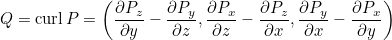
This function is meaningful for 3-D polynomials.
Example :
TinyVector<MultivariatePolynomial<Real_wp>, 3> P, Q;

// P consists of 3-D polynomials
P(0).SetOrder(3, 2);
P(1).SetOrder(3, 1);
P(2).SetOrder(3, 4);

// we compute Q = curl(P)
GetCurlPolynomial(P, Q);
Location :
Share/MultivariatePolynomial.cxx
GetDivPolynomial
Syntax
void GetDivPolynomial(const TinyVector<MultivariatePolynomial, 3>& P, MultivariatePolynomial& Q);
This function computes the divergence of P and stores it in Q.
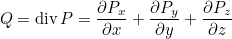
This function is meaningful for 3-D polynomials.
Example :
TinyVector<MultivariatePolynomial<Real_wp>, 3> P;

// P consists of 3-D polynomials
P(0).SetOrder(3, 2);
P(1).SetOrder(3, 1);
P(2).SetOrder(3, 4);

// we compute Q = div(P)
MultivariatePolynomial<Real_wp> Q;
GetDivPolynomial(P, Q);
Location :
Share/MultivariatePolynomial.cxx
IntegratePolynomial
Syntax
void IntegratePolynomial(const MultivariatePolynomial& P, MultivariatePolynomial& Q, int n);
This function computes the primitive of a polynomial with respect to a variable, the last argument corresponds to the variable number. This function is not implemented.
Example :
MultivariatePolynomial<Real_wp> P(2, 3), R, S;

// for 2-D polynomials, P(i, j) modifies the coefficient associated with x^i y^j
// P = 2 x^3 + 4 x^2 y - x y^2 + 5 y^3 + 3 x^2  - 4 x y - 3.2 y^2 + 5 x - 2.5 y + 8
P(3, 0) = 2.0; P(2, 1) = 4.0; P(1, 2) = -1.0; P(0, 3) = 5.0;
P(2, 0) = 3.0; P(1, 1) = -4.0; P(0, 2) = -3.2;
P(1, 0) = 5.0; P(0, 1) = -2.5;
P(0, 0) = 8.0;

// you can compute the primitive of P with respect to x
// x : 0, y : 1
IntegratePolynomial(P, R, 0);
Location :
Share/MultivariatePolynomial.cxx
Mlt
Syntax
void Mlt(T alpha, MultivariatePolynomial& P);
This function multiplies a polynomial by a scalar.
Example :
MultivariatePolynomial<Real_wp> P(2, 3);

// for 2-D polynomials, P(i, j) modifies the coefficient associated with x^i y^j
// P = 2 x^3 + 4 x^2 y - x y^2 + 5 y^3 + 3 x^2  - 4 x y - 3.2 y^2 + 5 x - 2.5 y + 8
P(3, 0) = 2.0; P(2, 1) = 4.0; P(1, 2) = -1.0; P(0, 3) = 5.0;
P(2, 0) = 3.0; P(1, 1) = -4.0; P(0, 2) = -3.2;
P(1, 0) = 5.0; P(0, 1) = -2.5;
P(0, 0) = 8.0;

// you can multiply P by a scalar
// equivalent to P = P*2.5
Mlt(Real_wp(2.5), P);
Location :
Share/MultivariatePolynomial.cxx
MltAdd
Syntax
void MltAdd(T alpha, const MultivariatePolynomial& P, const MultivariatePolynomial& Q, T beta, MultivariatePolynomial& R);
This function multiplies two polynomials P and Q and adds the result to R.
Example :
MultivariatePolynomial<Real_wp> P(2, 3), Q, R;

// for 2-D polynomials, P(i, j) modifies the coefficient associated with x^i y^j
// P = 2 x^3 + 4 x^2 y - x y^2 + 5 y^3 + 3 x^2  - 4 x y - 3.2 y^2 + 5 x - 2.5 y + 8
P(3, 0) = 2.0; P(2, 1) = 4.0; P(1, 2) = -1.0; P(0, 3) = 5.0;
P(2, 0) = 3.0; P(1, 1) = -4.0; P(0, 2) = -3.2;
P(1, 0) = 5.0; P(0, 1) = -2.5;
P(0, 0) = 8.0;

Q = P*P;

// equivalent to R = beta*R + alpha*P*Q
Real_wp alpha(2.2), beta(3.2);
MltAdd(alpha, P, Q, beta, R);
Location :
Share/MultivariatePolynomial.cxx
Add
Syntax
void Add(T alpha, const MultivariatePolynomial& P, MultivariatePolynomial& Q);
This function adds alpha*P to the polynomial Q.
Example :
MultivariatePolynomial<Real_wp> P(2, 3), Q;

// for 2-D polynomials, P(i, j) modifies the coefficient associated with x^i y^j
// P = 2 x^3 + 4 x^2 y - x y^2 + 5 y^3 + 3 x^2  - 4 x y - 3.2 y^2 + 5 x - 2.5 y + 8
P(3, 0) = 2.0; P(2, 1) = 4.0; P(1, 2) = -1.0; P(0, 3) = 5.0;
P(2, 0) = 3.0; P(1, 1) = -4.0; P(0, 2) = -3.2;
P(1, 0) = 5.0; P(0, 1) = -2.5;
P(0, 0) = 8.0;

// equivalent to Q = Q + alpha*P
Real_wp alpha = 2.4;
Add(alpha, P, Q);
Location :
Share/MultivariatePolynomial.cxx
IntegrateOnSimplex
Syntax
T IntegrateOnSimplex(const MultivariatePolynomial& P);
This function returns the integral of P over the unit simplex (in 2-D this simplex is the unit triangle, in 3-D the unit tetrahedron).
Example :
MultivariatePolynomial<Real_wp> P(2, 3), Q;

// for 2-D polynomials, P(i, j) modifies the coefficient associated with x^i y^j
// P = 2 x^3 + 4 x^2 y - x y^2 + 5 y^3 + 3 x^2  - 4 x y - 3.2 y^2 + 5 x - 2.5 y + 8
P(3, 0) = 2.0; P(2, 1) = 4.0; P(1, 2) = -1.0; P(0, 3) = 5.0;
P(2, 0) = 3.0; P(1, 1) = -4.0; P(0, 2) = -3.2;
P(1, 0) = 5.0; P(0, 1) = -2.5;
P(0, 0) = 8.0;

// intP = \int_0^1 \int_0^{1-x} P dy dx
Real_wp intP = IntegrateOnSimplex(P);
Location :
Share/MultivariatePolynomial.cxx
ScalePolynomVariable
Syntax
void ScalePolynomVariable(MultivariatePolynomial& P, T alpha);
This function computes the polynomial Q such that Q(x) = P(alpha x). P is overwritten with Q.
Example :
MultivariatePolynomial<Real_wp> P(2, 3), Q;

// for 2-D polynomials, P(i, j) modifies the coefficient associated with x^i y^j
// P = 2 x^3 + 4 x^2 y - x y^2 + 5 y^3 + 3 x^2  - 4 x y - 3.2 y^2 + 5 x - 2.5 y + 8
P(3, 0) = 2.0; P(2, 1) = 4.0; P(1, 2) = -1.0; P(0, 3) = 5.0;
P(2, 0) = 3.0; P(1, 1) = -4.0; P(0, 2) = -3.2;
P(1, 0) = 5.0; P(0, 1) = -2.5;
P(0, 0) = 8.0;

// P is replaced by P(alpha x)
Real_wp alpha = 2.5;
ScalePolynomVariable(P, alpha);
Location :
Share/MultivariatePolynomial.cxx
CompressPolynom
Syntax
void CompressPolynom(MultivariatePolynomial& P, T epsilon);
This function tries to reduce the degree of the polynomial P by removing coefficients smaller than epsilon.
Example :
MultivariatePolynomial<Real_wp> P(2, 2);

// P = 1e-10 x^2 - 2e-9 x y + 2e-10 y^2 + 2.0 x - 3.0 y - 5.0;
P(2, 0) = 1e-10; P(1, 1) = -2e-9; P(0, 2) = 2e-10;
P(1, 0) = 2.0; P(0, 1) = -3.0;
P(0, 0) = -5.0;

// here P will be reduced to a polynomial of degree 1
CompressPolynom(P, 1e-8);
Location :
Share/MultivariatePolynomial.cxx
OppositeX
Syntax
void OppositeX(MultivariatePolynomial& P);
This function replaces P(x, y, z) by P(-x, y, z). It is only implemented for 3-D polynomials.
Example :
MultivariatePolynomial<Real_wp> P(3, 2);

// P = 2 x^2 + 3 x y - 2.5 x z + 4 y^2 + 3.2 y z + 5 z^2 + 2 x - 1.5 y - 2.4 z + 8
P(2, 0, 0) = 2; P(1, 1, 0) = 3.0; P(1, 0, 1) = -2.5;
P(0, 2, 0) = 4.0; P(0, 1, 1) = 3.2; P(0, 0, 2) = 5;
P(1, 0, 0) = 2.0; P(0, 1, 0) = -1.5; P(0, 0, 1) = -2.4; P(0, 0, 0) = 8.0;

// P is replaced by P(-x, y, z)
// here it should give
// 2 x^2 - 3 x y + 2.5 x z + 4 y^2 + 3.2 y z + 5 z^2 - 2 x - 1.5 y - 2.4 z + 8
OppositeX(P);
Location :
Share/MultivariatePolynomial.cxx
OppositeY
Syntax
void OppositeY(MultivariatePolynomial& P);
This function replaces P(x, y, z) by P(x, -y, z). It is only implemented for 3-D polynomials.
Example :
MultivariatePolynomial<Real_wp> P(3, 2);

// P = 2 x^2 + 3 x y - 2.5 x z + 4 y^2 + 3.2 y z + 5 z^2 + 2 x - 1.5 y - 2.4 z + 8
P(2, 0, 0) = 2; P(1, 1, 0) = 3.0; P(1, 0, 1) = -2.5;
P(0, 2, 0) = 4.0; P(0, 1, 1) = 3.2; P(0, 0, 2) = 5;
P(1, 0, 0) = 2.0; P(0, 1, 0) = -1.5; P(0, 0, 1) = -2.4; P(0, 0, 0) = 8.0;

// P is replaced by P(x, -y, z)
// here it should give
// 2 x^2 - 3 x y - 2.5 x z + 4 y^2 - 3.2 y z + 5 z^2 + 2 x + 1.5 y - 2.4 z + 8
OppositeY(P);
Location :
Share/MultivariatePolynomial.cxx
PermuteXY
Syntax
void PermuteXY(MultivariatePolynomial& P);
This function replaces P(x, y, z) by P(y, x, z). It is only implemented for 3-D polynomials.
Example :
MultivariatePolynomial<Real_wp> P(3, 2);

// P = 2 x^2 + 3 x y - 2.5 x z + 4 y^2 + 3.2 y z + 5 z^2 + 2 x - 1.5 y - 2.4 z + 8
P(2, 0, 0) = 2; P(1, 1, 0) = 3.0; P(1, 0, 1) = -2.5;
P(0, 2, 0) = 4.0; P(0, 1, 1) = 3.2; P(0, 0, 2) = 5;
P(1, 0, 0) = 2.0; P(0, 1, 0) = -1.5; P(0, 0, 1) = -2.4; P(0, 0, 0) = 8.0;

// P is replaced by P(y, x, z)
// here it should give
// 2 y^2 + 3 x y - 2.5 y z + 4 x^2 + 3.2 x z + 5 z^2 + 2 y - 1.5 x - 2.4 z + 8
PermuteXY(P);
Location :
Share/MultivariatePolynomial.cxx
GenerateSymPol
Syntax
void GenerateSymPol(const MultivariatePolynomial& P, MultivariatePolynomial& Q, MultivariatePolynomial& R, MultivariatePolynomial& S);
This function computes P(-y, x, z), P(-x, -y, z) and P(y, -x, z) and stores them in Q, R and S. It is only implemented for 3-D polynomials.
Example :
MultivariatePolynomial<Real_wp> P(3, 2), Q, R, S;

// P = 2 x^2 + 3 x y - 2.5 x z + 4 y^2 + 3.2 y z + 5 z^2 + 2 x - 1.5 y - 2.4 z + 8
P(2, 0, 0) = 2; P(1, 1, 0) = 3.0; P(1, 0, 1) = -2.5;
P(0, 2, 0) = 4.0; P(0, 1, 1) = 3.2; P(0, 0, 2) = 5;
P(1, 0, 0) = 2.0; P(0, 1, 0) = -1.5; P(0, 0, 1) = -2.4; P(0, 0, 0) = 8.0;

GenerateSymPol(P, Q, R, S);
Location :
Share/MultivariatePolynomial.cxx
GenerateSym4_Vertices
Syntax
void GenerateSym4_Vertices(const MultivariatePolynomial& P, MultivariatePolynomial& Q, MultivariatePolynomial& R, MultivariatePolynomial& S);
This function computes P(-x, y, z), P(-x, -y, z) and P(x, -y, z) and stores them in Q, R and S. It is only implemented for 3-D polynomials.
Example :
MultivariatePolynomial<Real_wp> P(3, 2), Q, R, S;

// P = 2 x^2 + 3 x y - 2.5 x z + 4 y^2 + 3.2 y z + 5 z^2 + 2 x - 1.5 y - 2.4 z + 8
P(2, 0, 0) = 2; P(1, 1, 0) = 3.0; P(1, 0, 1) = -2.5;
P(0, 2, 0) = 4.0; P(0, 1, 1) = 3.2; P(0, 0, 2) = 5;
P(1, 0, 0) = 2.0; P(0, 1, 0) = -1.5; P(0, 0, 1) = -2.4; P(0, 0, 0) = 8.0;

GenerateSym4_Vertices(P, Q, R, S);
Location :
Share/MultivariatePolynomial.cxx
GenerateSym4_Edges
Syntax
void GenerateSym4_Edges(const MultivariatePolynomial& P, MultivariatePolynomial& Q, MultivariatePolynomial& R, MultivariatePolynomial& S);
This function computes P(x, -y, z), P(-y, x, z) and P(y, -x, z) and stores them in Q, R and S. It is only implemented for 3-D polynomials.
Example :
MultivariatePolynomial<Real_wp> P(3, 2), Q, R, S;

// P = 2 x^2 + 3 x y - 2.5 x z + 4 y^2 + 3.2 y z + 5 z^2 + 2 x - 1.5 y - 2.4 z + 8
P(2, 0, 0) = 2; P(1, 1, 0) = 3.0; P(1, 0, 1) = -2.5;
P(0, 2, 0) = 4.0; P(0, 1, 1) = 3.2; P(0, 0, 2) = 5;
P(1, 0, 0) = 2.0; P(0, 1, 0) = -1.5; P(0, 0, 1) = -2.4; P(0, 0, 0) = 8.0;

GenerateSym4_Edges(P, Q, R, S);
Location :
Share/MultivariatePolynomial.cxx
GenerateSym8
Syntax
  void GenerateSym8(const MultivariatePolynomial& P, MultivariatePolynomial& Q, MultivariatePolynomial& R, MultivariatePolynomial& S,
MultivariatePolynomial& T, MultivariatePolynomial& U, MultivariatePolynomial& V, MultivariatePolynomial& W);
This function computes P(-x, y, z), P(-x, -y, z), P(x, -y, z), P(-y, x, z), P(-y, -x, z), P(y, -x, z) and P(y, x, z) and stores them in Q, R, S, T, U, V and W. It is only implemented for 3-D polynomials.
Example :
MultivariatePolynomial<Real_wp> P(3, 2), Q, R, S, T, U, V, W;

// P = 2 x^2 + 3 x y - 2.5 x z + 4 y^2 + 3.2 y z + 5 z^2 + 2 x - 1.5 y - 2.4 z + 8
P(2, 0, 0) = 2; P(1, 1, 0) = 3.0; P(1, 0, 1) = -2.5;
P(0, 2, 0) = 4.0; P(0, 1, 1) = 3.2; P(0, 0, 2) = 5;
P(1, 0, 0) = 2.0; P(0, 1, 0) = -1.5; P(0, 0, 1) = -2.4; P(0, 0, 0) = 8.0;

GenerateSym8(P, Q, R, S, T, U, V, W);