Linearized Euler equation and Galbrun equations in time-harmonic or time-domain

These equations are modelling the propagation of acoustic waves in presence of flow (think for instance of the sound produced by an aircraft). We are only using Discontinuous Galerkin method to solve these equations since the functional spaces where the solution lies in, are not standard. We list here the partial differential equations solved by Montjoie. For the underlying variational formulations, we refer the reader to the general section devoted to equations solved in Montjoie

Linearized Euler equations

With the variables:

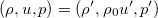
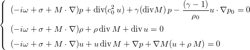
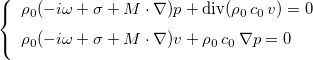
where are the perturbations of the density, flow and pressure, the Linearized Euler Equations (LEE) are given as:

are the background density, flow velocity, pressure and sound speed. These values are given in the datafile through MateriauDielec :

MateriauDielec = 1 ISOTROPE ux0 uy0 sigma rho0 c0 p0

is a damping coefficient. The coefficient is defined by the relation

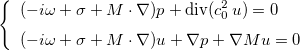
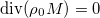
LEE equations are implemented in the class HarmonicLinearizedEulerEquation (file AeroAcoustic.hxx) for time-harmonic resolution, and in the class TimeLinearizedEulerEquation for time-domain resolution. When the density is uniform, the unknown can be removed and we obtain what we call simplified Linearized Euler equations :

The steady flow (M, ρ₀, p₀, c₀) and damping σ are provided through field MateriauDielec :

# MateriauDielec = ref ISOTROPE Mx My sigma rh0 c0 p0
MateriauDielec = 1 ISOTROPE 0.5 0.0 0.1 1.0 2.0  1.0

Of course you can specify non-uniform flow as explained in the description of MateriauDielec field.

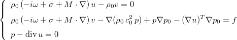
These simplified Linearized Euler Equations can be solved in time-harmonic domain (class HarmonicAeroAcousticEquation in file Aeroacoustic.hxx) and in time-domain (class TimeAeroAcousticEquation). In these equations, when the term is neglected, we obtain the Bogey-Bailly-Juve model

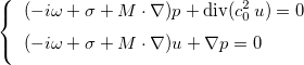
This model does not exhibit instabilities (such as Kevin-Helmholtz instabilities). In order to use this model, you have to write :

EnergyConservingAeroacousticModel = BogeyBaillyJuve

Another approximate model that leads to skew-symmetric stiffness matrix is given as:

This model is triggered if the data file contains the line:

EnergyConservingAeroacousticModel = YES

The approximate stiffness matrix (due to numerical integration) is skew-symmetric if the data file has a line

ExactIntegration = NO

However if the quadrature rules are accurate enough (such as Gauss-Legendre rules), you might set:

ExactIntegration = YES

In that case, the matrix-vector product should be more efficient. In the last conservative model, it is assumed that the steady flow satisfies the relation

The following boundary conditions are available for the different models presented above :

Dirichlet condition: . This condition can only be applied if the flow satisfies
Neumann condition: . This condition can only be applied if the flow satisfies
Absorbing condition: this condition is a first-order absorbing boundary condition. It can be applied to a boundary where the flow is uniform.

PML layers can also be added in time-harmonic domain if the flow is uniform on the extern boundary. Since no specific care is devoted to these PML, they should not be used in time domain since instabilities would arise.

Galbrun equations

An alternative model for aeroacoustics is Galbrun equation, which can be written as

This equation can be solved in time-harmonic domain with the following set of equations (class HarmonicGalbrunEquation) :

This set of equations can't be used in time-domain (not stable), we rather use the following set of equations (class HarmonicGalbrunEquationDG) :

In time-domain, the class TimeGalbrunEquation is using this formulation. Second-order formulation can also be used (but in time-harmonic domain only) with class HarmonicGalbrunEquationSipg, solving directly :

The following boundary conditions are implemented for Galbrun's equations:

Dirichlet condition: . This condition can only be applied if the flow satisfies
The second condition on p₀ means that the pressure must be constant on the boundary.
Neumann condition: . This condition can only be applied if the flow satisfies
Absorbing condition: this condition is a first-order absorbing boundary condition. This condition can only be applied if the flow satisfies