Data files in Montjoie
The data files are denoted with the extension .ini, but this extension is not mandatory, but useful in order to distinguish data files from other files. The data file consists of a sequence of entries of the type :
# My comment
Keyword1 = value1 value2 value3 \
       value4 value5
Keyword2 = value1 value2
As you noticed, each entry can be written on several lines by writing the special character \ at the end of each line. Values are separated by the space character. We encourage the user to start from a data file of the directory example, where all non-regression tests are present, and illustrate the solved equations. The data files present in the folder example should not be modified since these files are used to launch non-regression tests.
We detail here the list of present keywords in the data file, with examples and illustrations. We can classify them according to the class where these keywords are implemented. In all the classes, the treatment of the data file is performed by the method SetInputData (of a class deriving from InputDataProblem_Base) which looks like
void SetInputData(const string& description_field, const VectSring& parameters)
{
  if (description_field == "Frequency")
    {
      frequency = to_num<Real_wp>(parameters(0));
    }
  else if (description_field == "Polarization")
    {
       ...
    }
}
It is easy to add a new keyword in the data file by overloading this method SetInputData (if not present in the desired class) before the final definition of EllipticProblem (or HyperbolicProblem). The reading of the data file is actually performed by the function ReadInputFile which calls the method SetInputData for each entry of the data file.
Functions related to data files
| ReadInputFile | reads a data file to modify attributes of a class |
| ReadLinesFile | reads all the lines of an input file |
| SetInputData | modifies class for a given entry of the data file |
Below, a non-exhaustive list of keywords is available.
Keywords related to finite element problems :
| TypeElement | sets the finite element to use |
| TypeEquation | sets the equation to be solved |
| Adimensionalization | sets the type of adimensionalization performed |
| Frequency | frequency/pulsation of the problem |
| PhysicalFrequency | frequency for electromagnetic problems |
| Wavelength | wavelength for electromagnetic problems |
| WavelengthAdim | Units used in the mesh |
| IncidentAngle | incidence angle for incident wave if any |
| Polarization | polarization of the source |
| OriginePhase | point where the phase of incident wave is equal to 0. |
| ReferenceInfinity | reference associated with the infinite homogeneous medium |
Keywords related to mesh
| OrderGeometry | Order of geometric approximation |
| OrderDiscretization | Order of approximation |
| FileMesh | File name of the mesh or predefined mesh generated by Montjoie |
| AdditionalMesh | Other meshes can be specified there but won't be used |
| SaveSplitDomain | The mesh partitioning is saved in a binary file |
| SplitDomain | Algorithm for mesh partitioning used for parallel implementation |
| TypeMesh | type of elements for regular meshes (hexa, tetra, pyramids, wedges) |
| MeshPath | Directory where meshes will be read |
| IrregularMesh | Double-splitting to generate bad-quality meshes |
| SlightModificationOnRegularMesh | a regular mesh is slightly modified to obtain non-affine elements |
| RefinementVertex | Refinement around a vertex for 2-D meshes |
| AddVertex | inserts a new vertex for 2-D meshes |
| ThresholdMesh | modifies the threshold for meshes |
| TypeCurve | Type of curved surface (sphere, cylinder, cone ?) |
Keywords related to the solved equations
| MateriauDielec | Definition of physical properties of a domain |
| PhysicalMedia | Definition of a physical index |
| ExactIntegration | Is exact integration used ? (used by aeroacoustics) |
| MixedFormulation | Use of a mixed formulation ? |
| PenalizationDG | Penalty parameters that provide more stability when negative |
| CoefficientPenalization | changes the strategy for the coefficient in penalty terms |
Keywords related to boundary conditions
| PointDirichlet | Adds a node where dirichlet condition will be enforced |
| ModifiedImpedance | Modifies coefficient to improve first-order absorbing boundary condition |
| OrderAbsorbingBoundaryCondition | Order related to absorbing boundary condition |
| OrderHighConductivityBoundaryCondition | Order related to high conductivity boundary condition |
| Exit_IfNo_BoundaryCondition | Possibility to continue simulation when no boundary condition is specified |
| ConditionReference | Boundary condition associated to a referenced boundary of the mesh |
| ForceDirichletSymmetry | forces a symmetric Dirichlet condition |
| DirichletCoefMatrix | sets the coefficient on the diagonal of the matrix for Dirichlet dofs |
| StorageModes | the Fourier modes of the solution can be stored or not |
| NbModesPeriodic | the user provides the number of Fourier modes to compute |
| UseSameDofsForPeriodicCondition | uses same dof numbers for a periodic condition ? |
Keywords related to PML layers
| DampingPML | Damping factor inside PML |
| TransverseDampingPML | transverse damping factor inside PML |
| AddPML | PML layers can be added around the computational domain |
Keywords related to sparse linear solver
| Smoother | Type of smoother used in multigrid iteration |
| DampingParameters | Parameter alpha used in most of preconditioners. For complex problems like Helmholtz equation, an imaginary part is necessary. |
| DirectSolver | Direct solver for the coarsest level of multigrid preconditioning |
| NumberMaxIterations | Maximum number of iterations for the iterative solver |
| Tolerance | stopping criterion used by the iterative solver |
| TypeResolution | Type of solver (direct or iterative) and associated preconditioning, if any |
| TypeSolver | Type of solver (simplified version) |
| PivotThreshold | modifies the threshold used to perform pivoting |
| NbThreadsPerNode | sets the number of threads to use per MPI process |
| EstimationConditionNumber | computes an estimate of condition number of finite element matrix |
| StaticCondensation | internal degrees of freedom are removed by static condensation |
| ScalingMatrix | scales the finite element matrix before factorization |
| MumpsMemoryCoefficient | chooses different parameters for usage memory in Mumps |
Keywords related to eigenvalue computations
| Eigenvalue | Specification of eigenvalues and eigenmodes to compute |
| EigenvalueTolerance | Stopping criterioon for the computation of eigenvalues |
| EigenvalueMaxNumberIterations | maximum number of iterations allowed to find the eigenvalues |
| UseCholeskyForEigenvalue | Cholesky factorization is used to reduce the generalized eigenvalue problem to a standard one |
| FileEigenvalue | Sets the file where eigenvalues are written. |
| EigenvalueSolver | sets the eigenvalue solver used to find eigenvalues |
Keywords related to the source
| TypeSource | source in space |
| ThresholdRhs | threshold used to discard a right hand side |
| InitialCondition | initial condition to unsteady problems |
| TemporalSource | source in time |
Keywords related to unsteady problems
| TimeStep | time step dt |
| TimeInterval | computation for t belonging to the interval [t0, tf] |
| RandomInitialCondition | sets an initial condition with very small random values |
| DisplayRate | number of iterations between each display |
| OrderTimeScheme | specification of time scheme |
| UseWarburtonTrick | uses Warburton's trick to save memory for curved tetrahedral in DG method |
| LoadReprise | loads data on the disk to resume time iterations |
| SaveReprise | saves data on the disk that can be used to resume the simulation later |
| PathReprise | Directory where the data used to resume the simulation is written |
| NormeMaxSolution | allowed maximal norm of the solution |
Keywords related to the computation of radar cross sections
| ParametersRCS | specification of radar cross section that will be computed |
| AngleRCS | angles for which you want to know radar cross section |
| FileRCS | file where radar cross section will be stored |
Keywords related to transparent condition
| TransparencyCondition | specification of transparent condition to use |
| ParamResolutionTransparency | additional parameters associated with transparent condition |
| TypeBody | Definition of a body contaning several references |
Various keywords
| ExplicitMatrixFEM | finite element matrix is computed explicitly ? |
| StorageMatrix | finite element matrix can be written on a file is asked |
| ThresholdMatrix | values below a given value are dropped |
| Seed | defines the random seed |
| NumberPhysicalMedia | defines the maximal media number |
| Timer | defines the timer to use to measure the computational time |
| NbProcessorsPerMode | specifies which processors should compute each mode |
| PrintLevel | Level of information to print |
| WriteQuadraturePoints | Writes quadrature points on a text file |
Keywords for targets migration and inv_harmonic
| DataFileExperiment | ini file for experimental data |
| DataFileSimulation | ini file for simulated data |
| TypeSourceLine | sources located on a line |
| TypeSourceCircle | sources located on a circle |
Keywords for aeroacoustics
| EnergyConservingAeroacousticModel | Model to use for aeroacoustics |
| DropUnstableTerms | Drops terms that are not stable for Galbrun's equations |
| ApplyConvectiveCorrectionSource | Applies convective derivative to the source |
| ForceFlowNeumann | enforces neumann condition in given stationary flow |
Keywords for axisymmetric targets
| NumberModes | number of Fourier modes (in teta) for axisymmetric problems |
| ForceDiagonalMass | forces mass lumping for axisymmetric Helmholtz |
Keywords for acoustics (and Helmholtz)
| AddFlowTerm | adds a convection term in Helmholtz equation. |
| AddSlot | adds a thin slot in the computational domain for 2-D Helmholtz equation. |
| ModelSlot | selects model used for thin slots and 2-D Helmholtz equation |
| CalculEnveloppe | the enveloppe is computed ? |
| FormulationAxisymmetric | selects a different variational formulation for the target helm_axi |
| TimeReversal | parameters for time reversal experiences |
Keywords for time-harmonic Maxwell's equations
| FileCoefficientsQ | computes coefficients qi for each element. |
| ModifiedFormulation | uses a modified formulation for maxwell_axi |
| OutputHy | writes Hy on a surface |
Keywords for Elastodynamics
| DisplayStress | displays or no the stress sigma |
Keywords for Reissner-Mindlin
| ThicknessPlate | Thickness of the plate for Reissner-Mindlin model |
Keywords for outputs
| FileOutputGrille | name of the files containing diffracted and total field |
| FileOutputGrille3D | Idem |
| FileOutputPlane | Idem |
| FileOutputPlaneAxi | Idem |
| FileOutputLine | Idem |
| FileOutputLineAxi | Idem |
| FileOutputCircle | Idem |
| FileOutputCircleAxi | Idem |
| FileOutputPointsFile | Idem |
| FileOutputPointsFile | Idem |
| FileOutputMeshSurfacic | Idem |
| FileOutputMeshVolumetric | Idem |
| FileOutputPoint | name of the files containing seismogramms |
| FileOutputPointAxi | name of the files containing seismogramms |
| ParametersOutputGrille | snapshots in interval [t0, tf] each dt |
| ParametersOutputGrille3D | Idem |
| ParametersOutputPlane | Idem |
| ParametersOutputPlaneAxi | Idem |
| ParametersOutputLine | Idem |
| ParametersOutputLineAxi | Idem |
| ParametersOutputCircle | Idem |
| ParametersOutputCircleAxi | Idem |
| ParametersOutputPoint | Idem |
| ParametersOutputPointAxi | Idem |
| ParametersOutputMeshSurfacic | Idem |
| ParametersOutputMeshVolumetric | Idem |
| SismoGrille | Snapshot on three cartesian planes |
| SismoGrille3D | Snapshot on 3-D regular grid |
| SismoPlane | Snapshot on a plane |
| SismoPlaneAxi | Snapshot on a 3-D plane |
| SismoLine | Snapshot on a line |
| SismoLineAxi | Snapshot on a 3-D line |
| SismoCircle | Snapshot on a circle |
| SismoCircleAxi | Snapshot on a 3-D circle |
| SismoPoint | Seismogramms on points |
| SismoPointAxi | Seismogramms on 3-D points |
| SismoPointsFile | Snapshot on points provided by a text file |
| SismoPointsFileAxi | Snapshot on 3-D points provided by a text file |
| SismoMeshSurfacic | Snapshot on a surfacic mesh |
| SismoMeshVolumetric | Snapshot on a volume mesh |
| SismoOutsidePoints | Snapshot on far points (located outside the mesh) |
| OutputFormat | Format of output files |
| DirectoryOutput | Directory where output files will be written |
| ElectricOrMagnetic | component of the field which will be written on output files |
| FineMeshLobatto | subdivided-mesh based on nodal points instead of regular points ? |
| WriteSolutionQuadrature | writes the solution on quadrature points of the mesh |
| MovePointsSurface | outputs on surface meshes consist of translated points |
| NonLinearSolver | Solver used to invert transformation Fi |
ReadInputFile
Syntax :
  void ReadInputFile(const string& file_name, InputDataProblem_Base& var);
  void ReadInputFile(const Vector<string>& all_lines, InputDataProblem_Base& var);
This method reads a data file by calling the virtual method SetInputData (which is therefore overloaded in a derived class of type InputDataProblem_Base) for each entry of the data file.
Example :
// your own class that derives from InputDataProblem_Base
class MyClass : public InputDataProblem_Base
{
  int my_variable;

  public :
  // your own definition of SetInputData
  void SetInputData(const string& keyword, const Vector<string>& parameters)
  {
     // for each keyword -> your own treatment
     if (keyword == "MyKeyword")
       {
         // example of treatment
         my_variable = to_num<int>(parameters(0));
       }
  }

};

// in main function for example, you can call ReadInputFile
int main ()
{
  // first solution : the data file is read and treated
  MyClass var;
  ReadInputFile(string("datafile.ini"), var);

  // another solution is to read first all the lines of the input file
  // and store these lines :
  Vector<string> all_lines;

  ReadLinesFile(string("datafile.ini"), all_lines);

  // then you can treat these lines afterwards
  ReadInputFile(all_lines, var);
}
Related topics :
Location :
ReadLinesFile
Syntax :
  void ReadLinesFile(const string& file_name, Vector<string>& all_lines);
  void ReadLinesFile(const string& file_name, Vector<string>& all_lines, const MPI::Comm& comm);
This method reads a data file and stores the lines in the second argument. The third argument is optional and useful for parallel execution. If the third argument is not provided, all processors will read the same data file. If the communicator is provided, only the root processor (of rank 0) will read the data file and sends the lines to other processors through the communicator.
Example :
// in main function for example, you can call ReadInputFile
int main ()
{
  // first solution : the data file is read and treated
  MyClass var;
  ReadInputFile(string("datafile.ini"), var);

  // another solution is to read first all the lines of the input file
  // and store these lines :
  Vector<string> all_lines;

  // if you want that only one processor reads the data file
  // you specify a communicator
  ReadLinesFile(string("datafile.ini"), all_lines, MPI::COMM_WORLD);

  // then you can treat these lines afterwards
  ReadInputFile(all_lines, var);
}
Related topics :
Location :
SetInputData
Syntax :
void SetInputData(const string& keyword, const Vector<string>& param);
This method deals with an entry of the data file. The first argument is the keyword associated with the entry, and the second argument stores all the parameters (separated by space characters) after the sign equal.
Example :
// usually it is called by ReadInputFile, but you can also call it alone
EllipticProblem<TypeEquation> var;
Vector<string> param(3);
param(0) = "34";
param(1) = "YES";
param(2) = "5.0";
var.SetInputData(string("StandardKeyword"), param);
Related topics :
Location :
FiniteElement/PointsReference.cxx
Harmonic/BoundaryConditionHarmonic.cxx
Harmonic/DistributedProblem.cxx
Harmonic/TransparencyCondition.cxx
Mesh/MeshBoundaries.cxx
Harmonic/VarAxisymProblem.cxx
Harmonic/VarGeometryProblem.cxx
Harmonic/VarMigration.cxx
Harmonic/VarProblemBase.cxx
Elliptic/PhysicalProperty.cxx
Mesh/NumberMesh.cxx
Instationary/TimeSchemes.cxx
Instationary/VarInstationary.cxx
Mesh/MeshBase.cxx
Mesh/Mesh2D.cxx
Mesh/Mesh3D.cxx
Mesh/MeshBoundaries.cxx
Output/GridInterpolation.cxx
Output/OutputHarmonic.cxx
Solver/SolveSystem.cxx
Solver/SolveHarmonic.cxx
Solver/Preconditioner.cxx
Source/DefineSourceElliptic.cxx
TypeElement
Syntax :
TypeElement = name_element
This line specifies which finite element is used. 1-D finite elements are the following ones:
- EDGE_GAUSS: Gauss-Lobatto points are used as interpolation points while Gauss points are used as quadrature points
- EDGE_LOBATTO : Gauss-Lobatto points are used both for interpolation and quadrature (this finite element implies a mass lumping, ie a diagonal mass matrix). This is usually the preferred finite element in 1-D.
- EDGE_HIERARCHIC : Hierarchical basis functions are used (with Jacobi polynomials).
2-D scalar finite elements are the following ones (names in parenthesis are equivalent):
- TRIANGLE_CLASSICAL (TRIANGLE_DG_LOBATTO_GAUSS) : Gauss-Lobatto points are used as interpolation points for quadrilaterals, and Hesthaven's points for triangles. Quadrature rules are based on Gauss points for quadrangles (and Dunavant rules for triangles).
- TRIANGLE_LOBATTO (QUADRANGLE_LOBATTO, TRIANGLE_DG_LOBATTO) : Gauss-Lobatto points are used both for interpolation and quadrature for quadrilaterals. Triangular elements are similar to TRIANGLE_CLASSICAL. If the mesh contains only quadrilaterals, the mass matrix is diagonal.
- TRIANGLE_HIERARCHIC : Hierarchical basis functions are used for quadrilaterals and triangles (based on Jacobi polynomials). The main advantage of this finite element is that it allows variable order with continuous formulation.
- QUADRANGLE_DG_GAUSS (TRIANGLE_DG_CLASSICAL) : Gauss points are used both for interpolation and quadrature for quadrilaterals. Triangular elements are the same as for TRIANGLE_CLASSICAL. This finite element is available only for discontinuous Galerkin formulation.
- TRIANGLE_DG_ORTHO : orthogonal basis functions are used for triangles (Gauss points for quadrilaterals). The mass matrix for triangular straight elements is diagonal. This finite element is available only for discontinuous Galerkin formulation.
3-D scalar finite elements are the following ones (names in parenthesis are equivalent):
- TETRAHEDRON_CLASSICAL (TETRAHEDRON_DG_LOBATTO_GAUSS) : Gauss-Lobatto points are used as interpolation points for hexahedra, Hesthaven's points for tetrahedra, and compliant interpolation points for prisms and pyramids. Quadrature rules are based on Gauss points for hexahedra.
- TETRAHEDRON_LOBATTO (HEXAHEDRON_LOBATTO, TETRAHEDRON_DG_LOBATTO) : Gauss-Lobatto points are used both for interpolation and quadrature for hexahedron. Tetrahedral, prismatic and pyramidal elements are similar to TETRAHEDRON_CLASSICAL. If the mesh contains only hexahedra, the mass matrix is diagonal.
- TETRAHEDRON_HIERARCHIC : Hierarchical basis functions are used for hexahedra, wedges, pyramids and tetrahedra (based on Jacobi polynomials). The main advantage of this finite element is that it allows variable order with continuous formulation.
- HEXAHEDRON_DG_GAUSS (TETRAHEDRON_DG_CLASSICAL) : Gauss points are used both for interpolation and quadrature for hexahedra. Tetrahedral, prismatic and pyramidal elements are similar to TETRAHEDRON_CLASSICAL. This finite element is available only for discontinuous Galerkin formulation.
- TETRAHEDRON_DG_ORTHO : orthogonal basis functions are used for all elements (Gauss points for hexahedra). The mass matrix for straight elements is diagonal. This finite element is available only for discontinuous Galerkin formulation.
- TETRAHEDRON_DG_LEGENDRE : orthogonal basis functions are used
for all elements (Gauss points for hexahedra). The mass matrix for
straight elements is diagonal. The difference with
TETRAHEDRON_DG_ORTHO is that the polynomial space for all elements
is
 (i.e. polynomial of total degree less or equal to r) instead of the
optimal
finite element space (see Bergot's thesis). As a result, this finite
element would not converge nicely for non-affine elements, and should
be used cautiously. This finite element is
available only for discontinuous Galerkin formulation.
(i.e. polynomial of total degree less or equal to r) instead of the
optimal
finite element space (see Bergot's thesis). As a result, this finite
element would not converge nicely for non-affine elements, and should
be used cautiously. This finite element is
available only for discontinuous Galerkin formulation. - TETRAHEDRON_DG_OPTIMAL : orthogonal basis functions are used for pyramidal, prismatic and hexahedral elements whereas nodal basis functions (as for TETRAHEDRON_CLASSICAL) are used for tetrahedron. Usually this mix of elements is the most efficient.
2-D edge finite elements are the following ones (for example used in targets maxwell2D or mode_maxwell):
- TRIANGLE_FIRST_FAMILY (QUADRANGLE_FIRST_FAMILY) : nodal edge elements for triangles/quadrilaterals. The polynomial generated space is the Nedelec's first family. A special quadrature is used for quadrilaterals.
- QUADRANGLE_GAUSS_FIRST_FAMILY nodal edge elements for triangles/quadrilaterals. The polynomial generated space is the Nedelec's first family. Gauss quadrature is used for quadrilaterals.
- TRIANGLE_OPTIMAL_FIRST_FAMILY : nodal edge elements for triangles/quadrilaterals. The polynomial generated space is the optimal Nedelec's first family as detailed in Bergot's thesis.
- TRIANGLE_SECOND_FAMILY (QUADRANGLE_HCURL_LOBATTO) : nodal edge elements for triangles/quadrilaterals. The polynomial generated space is the Nedelec's second family. This family generates spurious modes if the mesh contains quadrilaterals.
- TRIANGLE_HP_FIRST_FAMILY : hierarchical edge elements for triangles/quadrilaterals. The polynomial generated space is the Nedelec's first family.
- TRIANGLE_OPTIMAL_HP_FIRST_FAMILY : hierarchical edge elements for triangles/quadrilaterals. The polynomial generated space is the optimal Nedelec's first family.
3-D edge finite elements are the following ones (for example used in target maxwell3D):
- TETRAHEDRON_FIRST_FAMILY (HEXAHEDRON_FIRST_FAMILY) : nodal edge elements for tetrahedra, pyramids, wedges and hexahedra. The finite element space is the Nedelec's first family.
- TETRAHEDRON_OPTIMAL_FIRST_FAMILY : nodal edge elements for tetrahedra, pyramids, wedges and hexahedra. The finite element space is the optimal Nedelec's first family as detailed in Bergot's thesis.
- HEXAHEDRON_HCURL_LOBATTO (QUADRANGLE_HCURL_LOBATTO) : nodal edge elements for hexahedra only (the mesh should not contain tetrahedra, prisms or pyramids). The polynomial generated space is the Nedelec's second family. This family generates spurious modes.
- TETRAHEDRON_HP_FIRST_FAMILY : hierarchical edge elements for tetrahedra, pyramids, wedges and hexahedra. The finite element space is the Nedelec's first family.
- TETRAHEDRON_OPTIMAL_HP_FIRST_FAMILY : hierarchical edge elements for tetrahedra, pyramids, wedges and hexahedra. The finite element space is the optimal Nedelec's first family.
2-D facet finite elements (for H(div) space) are the following ones (for example used in target helm_div):
- TRIANGLE_FIRST_FAMILY (QUADRANGLE_FIRST_FAMILY) : nodal facet elements for triangles/quadrilaterals. The polynomial generated space is the Nedelec's first family.
- TRIANGLE_OPTIMAL_FIRST_FAMILY : nodal facet elements for triangles/quadrilaterals. The polynomial generated space is the optimal Nedelec's first family as detailed in Bergot's thesis.
- TRIANGLE_HP_FIRST_FAMILY : hierarchical facet elements for triangles/quadrilaterals. The polynomial generated space is the Nedelec's first family.
- TRIANGLE_OPTIMAL_HP_FIRST_FAMILY : hierarchical facet elements for triangles/quadrilaterals. The polynomial generated space is the optimal Nedelec's first family.
3-D facet finite elements (for H(div)) are the following ones (for example used in target helm_div):
- TETRAHEDRON_FIRST_FAMILY : nodal facet elements for tetrahedra, pyramids, wedges and hexahedra. The finite element space is the Nedelec's first family.
- TETRAHEDRON_OPTIMAL_FIRST_FAMILY : nodal facet elements for tetrahedra, pyramids, wedges and hexahedra. The finite element space is the optimal Nedelec's first family as detailed in Bergot's thesis.
- TETRAHEDRON_HP_FIRST_FAMILY : hierarchical facet elements for tetrahedra, pyramids, wedges and hexahedra. The finite element space is the Nedelec's first family.
- TETRAHEDRON_OPTIMAL_HP_FIRST_FAMILY : hierarchical facet elements for tetrahedra, pyramids, wedges and hexahedra. The finite element space is the optimal Nedelec's first family.
For the target maxwell_axi, a mix of edge elements and nodal elements is used and called QUADRANGLE_HCURL_AXI.
Example :
TypeElement = TRIANGLE_LOBATTO
Location :
Elliptic/Maxwell/PhysicalConstant.cxx
TypeEquation
Syntax :
TypeEquation = name_equation
This line specifies which equation is solved by the code. Actually this field is used only for some targets. As you noticed, for most of targets, the equation is already uniquely associated with the name of the target.
Example :
# to use Discontinuous Galerking for acoustics :
TypeEquation = ACOUSTIC_DG
Location :
Elliptic/Maxwell/PhysicalConstant.cxx
Adimensionalization
Syntax :
Adimensionalization = YES
Adimensionalization = NO
Adimensionalization = ONE
This line is used to specify how equations are adimensionalized. The avaible choices are the following ones:
- NO : no adimensionalization is performed, the user must provide physical values for all parameters (time step, frequency, etc).
- YES:an adimensionalization is performed, but there should not be any impact on the user. The user must provide physical values, these values are changed inside the code, and outputs are modified in order to contain physical values.
- ONE : the adimensionalization is performed by the user who provides adimensionalized values. With this mode, the velocity and wavelength at infinity are usually assumed to be equal to 1.
The default adimensionalization mode is ONE.
Example :
Adimensionalization = YES
Location :
Elliptic/Maxwell/PhysicalConstant.cxx
Seed
Syntax :
Seed = n
This line should be the first line of the input file if you want to specify a random seed that will be common to all processors. This seed is used for random Gaussian sources.
Example :
Seed = 103
Location :
Elliptic/Maxwell/PhysicalConstant.cxx
NumberPhysicalMedia
Syntax :
NumberPhysicalMedia = N
The number N is the maximal number for the volume references in the mesh. In Gmsh, it would correspond to the maximum number of Physical Surface (in 2-D) and Physical Volume (in 3-D). The physical indexes (such as epsilon, mu, sigma, etc) are stored in an array whose dimension is equal to this number. The default value is 20.
Example :
# if you have a physical volume of reference 100 (maximum value):
NumberPhysicalMedia = 100
Location :
Elliptic/Maxwell/PhysicalConstant.cxx
Timer
Syntax :
Timer = Name
You can select the timer to use for the measurement of computation time. You can choose between Accurate, Real or Basic. The default timer is Real if you whave compiled with the flag MONTJOIE_WITH_REAL_TIMING, Basic otherwise. Accurate timer is based on the C function getrusage, Real timer is based on C function clock_gettime while Basic timer is based on C function clock.
Example :
# if you want to use real timing
Timer = Real
Location :
Elliptic/Maxwell/PhysicalConstant.cxx
Frequency
Syntax :
Frequency = freq omega
You can specify either a frequency freq or a pulsation omega. The resulting pulsation is equal to freq*2*pi + omega. In case of adimensionalization, this frequency is multiplied by L/c where L is a characteristic wavelength and c the speed of light.
Example :
# For a frequency equal to 1 (then pulsation = 2 pi)
Frequency = 1.0  0

# For a pulsation equal to 10 (then frequency = 10/(2 pi) )
Frequency = 0  10.0
Related topics :
Location :
PhysicalFrequency
Syntax :
PhysicalFrequency = freq
For Helmholtz and Maxwell equations, we usually perform an adimensionalization so that a frequency equal to 1 corresponds in the physical space to a frequency approximatively equal to 300 Mhz. Therefore in this field, you can write the physical frequency (in Hz), and the conversion to adimensionalized frequency will be performed by dividing by the speed of light in free space.
Example :
# For a physical frequency equal to 2.5 Ghz
PhysicalFrequency = 2.5e9
Related topics :
time-harmonic maxwell equations
Location :
Wavelength, WaveLength
Syntax :
  WaveLength = lambda
  Wavelength = lambda
You can specify the wavelength, the frequency is therefore equal to L/lambda where L is the characteristic wavelength specified in the parameter WavelengthAdim.
Example :
# for a wavelength of 200nm :
Wavelength = 200e-9
Location :
WavelengthAdim
Syntax :
WavelengthAdim = L
You can specify the characteristic wavelength in this field. It represents the unit used in the mesh (a distance of 1 in the mesh represents L meters).
Example :
# if you have constructed your mesh with units of micrometers
Adimensionalization = YES
WavelengthAdim = 1e-6

# for a wavelength of 200nm :
Wavelength = 200e-9
Location :
IncidentAngle
Syntax :
IncidentAngle = teta phi
When the selected source is an incident plane wave, the incident angle is specified by these two angles in 3-D, and only by an angle in 2-D. The values are expressed in degrees. In 2-D the wave vector is equal to:
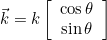
where k is the wave number. In 3-D the wave vector is given as:
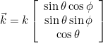
Example :
# In 3-D (or axisymmetric), you enter theta and phi
IncidentAngle = 90 90
Related topics :
Location :
Harmonic/VarGeometryProblem.cxx
Polarization
Syntax :
Polarization = p0 p1 p2 ... pk
When the spatial dependence of the source is scalar, the polarization is the direction of the source, i.e. the constant vector appearing in the source. The number of components of the polarization depends on the solved equation. For scalar equations like Helmholtz equation, this value has no meaning, whereas it is useful for vectorial equations (like Maxwell equations). The default value is the constant vector (1,0,0...,0). When a total or diffracted field is computed, this polarization is the polarization of the incident wave.
Example :
# For maxwell equations, three components
# and you can specify polarization along ey
Polarization = 0 1.0 0
Related topics :
Location :
Harmonic/VarGeometryProblem.cxx
UseWarburtonTrick
Syntax :
UseWarburtonTrick = YES
This trick can be used to reduce the storage for discontinuous Galerkin. Basis functions are transformed as :

such that the mass matrix no longer depends on the geometry. As a result, the inverse of the mass matrix is not stored. This trick is interesting for curved tetrahedral elements.
Example :
UseWarburtonTrick = YES
Location :
Harmonic/VarGeometryProblem.cxx
UseSameDofsForPeriodicCondition
Syntax :
UseSameDofsForPeriodicCondition = type
For periodic condition, you can choose to use same dof numbers for periodic dofs. With this choice, the finite element matrix is naturally symmetric. But you cannot have a quasi-periodic condition (used for PERIODIC_X boundary condition). For this kind of condition, it is better to use a strong formulation or a weak formulation. The choices are the following:
- YES : periodic dofs have the same numbers
- NO : periodic dofs have different numbers, and the relation ui = uj is set strongly in the finite element matrix (instead of rows). The finite element matrix is non-symmetric.
- WEAK : periodic dofs have different number and the periodic condition is enforced in the weak formulation. The finite element matrix is symmetric.
Example :
UseSameDofsForPeriodicCondition = WEAK
Location :
OriginePhase
Syntax :
OriginePhase = x0 y0 z0
For incident waves, the phase is equal to 1 at the origin O. You can set this origin at a different value from the default value (0,0,0).
Example :
# If you want the origin at (5, 0, 3)
OriginePhase = 5 0 3
Related topics :
Location :
Harmonic/VarAxisymProblem.cxx
Harmonic/VarGeometryProblem.cxx
ReferenceInfinity
Syntax :
ReferenceInfinity = ref
For incident waves, the infinite homogeneous media is often considered with physical indices (epsilon and mu) equal to 1. You can give the reference (in the mesh) for this infinite homogeneous media such that the wave number is correctly computed.
Example :
# if elements at infinity have reference 2
ReferenceInfinity = 2
Related topics :
Location :
Harmonic/VarGeometryProblem.cxx
OrderGeometry
Syntax :
OrderGeometry = order
By default, the same order is used both for geometry and finite element (isoparametric elements). However, you may want to specify different orders. Moreover, when you adopt a variable order strategy, you need to specify the order used to approximate geometry. Since the mesh uses classical nodal elements, a fixed order is used to describe curved elements.
Example :
# for example you use a variable order
OrderDiscretization = MEAN_EDGE AUTO 0.5

# you need to specify the order for the geometry
# otherwise a first-order approximation is used (linear elements)
OrderGeometry = 6
OrderDiscretization
Syntax :
OrderDiscretization = n
The order of approximation should be chosen depending on the mesh size and the wavelength. Usually, we will take 10 points per wavelength for a Q2 scheme and 7 points per wavelength for a Q7 scheme, i.e. the mesh size will be equal to the wavelength for an order of approximation equal to 7. Variable orders can also be specified (for Discontinuous Galerkin formulation or with hierarchical elements such as TRIANGLE_HIERARCHIC/TETRAHEDRON_HIERARCHIC). The attribution of an order to an element is purely geometric and based on this rule of thumb "10 points per wavelength". For each edge, an order r is attributed if the length of the edge is comprised between :
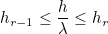
Here λ denotes the wavelength of the media (on this edge). When AUTO is provided, we take the following values for hr
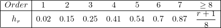
For example, it means that when there are more than 50 points per wavelength (the inverse of 0.02), a first-order is considered accurate enough and is chosen. Between 13.33 points and 50 points, a second-order is chosen, etc. You can replace AUTO with your own sequence of sizes hr.
Example :
# the same order 3 will be used for all elements
OrderDiscretization = 3

# a variable order will be used
# for faces/volumes, we take the maximum among edge lengths to determine the order
# the last parameter if here a coefficient used to refine in order when it is decreased
# 1.0 is the nominal value for 10 points per wavelength
OrderDiscretization = MAX_EDGE AUTO 0.5

# you can define your own sequence of h_r
# MEAN_EDGE : we take the mean edge length
# the coefficient is here placed at the beginning for a manual sequence
OrderDiscretization = MEAN_EDGE 0.5   0.01 0.1 0.2 0.3 0.4 0.55 0.7 0.9 1.1 1.3

# For high order, nodal triangles have the drawback that interpolation
# nodes are not present in the code
# You can either use a geometric order below 12 : (the geometry order is the second argument)
OrderDiscretization = 20 10

# if you are sure that the mesh only contains quad/hexa, you can inform the code with the keyword QUAD
OrderDiscretization = 20 QUAD
Related topics :
Location :
FileMesh
Syntax :
FileMesh = nom_fichier
FileMesh = nom_fichier REFINED n

# 2-D regular mesh
FileMesh = REGULAR nx xmin xmax ymin ymax ref ref1 ref2 ref3 ref4
FileMesh = REGULAR_ANISO nx ny xmin xmax ymin ymax ref ref1 ref2 ref3 ref4

# 3-D regular meshes
FileMesh = REGULAR nx xmin xmax ymin ymax zmin zmax ref ref1 ref2 ref3 ref4 ref5 ref6
FileMesh = REGULAR_ANISO nx ny nz xmin xmax ymin ymax zmin zmax ref ref1 ref2 ref3 ref4 ref5 ref6
FileMesh = SPHERE rmin rmax nb_points
FileMesh = SPHERE rmin rmax nb_points r0 r1 ... rk
FileMesh = SPHERE_CUBE rmin rmax nb_points
FileMesh = BALL rmin rmax nb_points ref REGULAR
FileMesh = BALL_CUBE rmin rmax nb_points ref REGULAR
FileMesh = EXTRUDE nb_layers z0 z1 ... zn nom_fichier AUTO \
           nb_ref_surf ref0 ref1 ref2 ... ref2n \
           nb_ref_vol ref0 ref1 ref2 ... refn
The file mesh can be either a file or a primitive (like a cube, sphere) for simple shapes. nom_fichier denotes the file name, the optional parameters "REFINED n" allows the user to split the initial mesh, each edge being divided into n small edges. This splitting procedure is implemented for hybrid meshes in 2-D and 3-D.
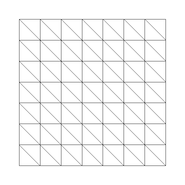
In 2-D, you can specify a rectangular domain [xmin, xmax] x [ymin, ymax] ( REGULAR ) with equally distributed points, nx is the number of points along x, the number of points along y is automatically computed. ref is the reference of the 2-D domain while ref1, ref2, ref3 and ref4 are the references of the four boundaries, respectively y = ymin, x = xmax, y = ymax and x = xmin. By default, the code computes automatically the number of points along y (by trying to have approximatively the same space step in x and y). If you want to enter manually nx and ny, you can use the keyword REGULAR_ANISO instead of REGULAR.
 |
 |
The two types of regular meshes in 2-D (REGULAR) with specifying TypeMesh = TRI or TypeMesh = QUAD
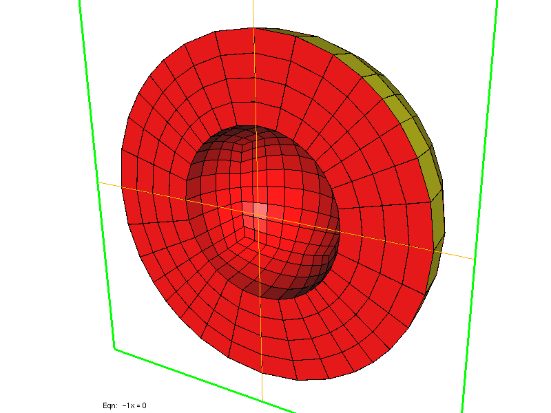
In 3-D, you can specify a parallelepiped [xmin, xmax] x [ymin, ymax] x [zmin, zmax], again you select only the number of points along x. ref is the reference of the 3-D domain, while ref1, ref2, ref3, ref4, ref5, ref6 are the references of the six boundaries, respectively x = xmin, y = ymin, z = zmin, z = zmax, y = ymax, x = xmax. The parameter SPHERE corresponds to spherical layers between an intern sphere of radius rmin (strictly positive) and extern sphere of radius rmax. nb_points is the number of points per unit, optional parameters r0, r1, ... rk are radius of intermediary spheres. The parameter SPHERE_CUBE provides same functionality as SPHERE except that the extern boundary is a cube, no intermediary layer is possible. You can also have the inside of the sphere meshed if you specify BALL (and BALL_CUBE if the extern boundary is a cube).
 |
 |
Several patterns for meshing an elementary cell (REGULAR).
 |
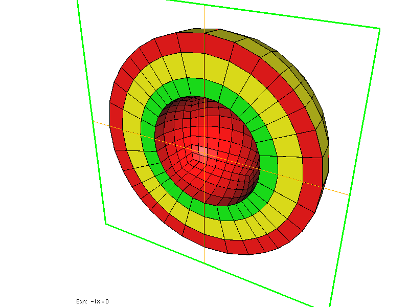 |
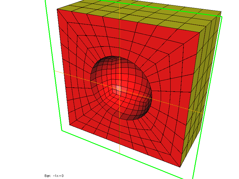 |
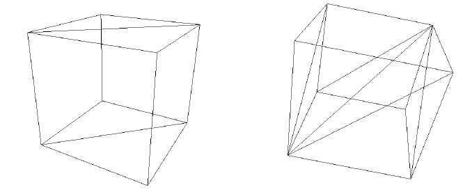
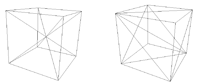
Two left meshes have been generated by using SPHERE, while right mesh has been generated by using SPHERE_CUBE.
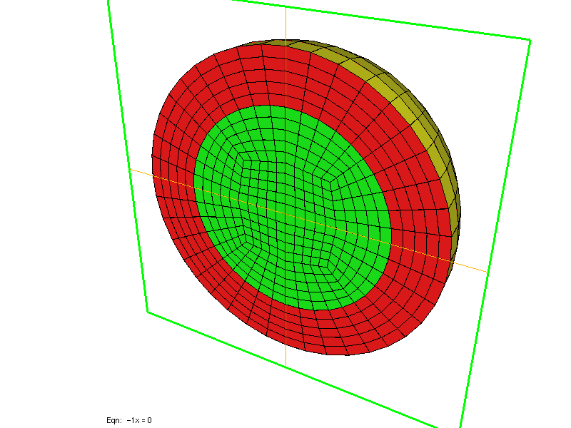 |
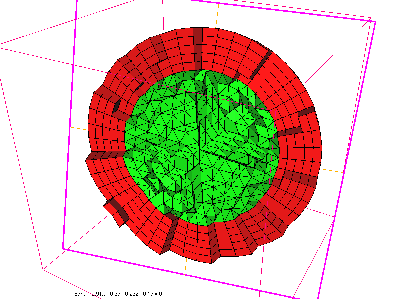 |
Meshes generated by using BALL, with TypeMesh = HEXA and TypeMesh = PYRAMID.
Finally, you can create a mesh by extruding a 2-D mesh along axis z (it will create hexahedra and wedges), intermediary layers can be inserted at z-coordinate z0, z1, z2 ..., zn. The initial 2-D mesh is read in the file whose name is nom_fichier. "AUTO" means here that the number of cells along z will be computed by evaluating the mesh step in 2-D, and trying to have the same mesh step for z. During the extrusion, you can change the references of lateral faces, by selecting appropriate ref0 ref1 ref2 ... refn, and the reference of top faces by chosing appropriate refn+1 ... ref2n. If a reference is set to 0, no referenced faces will be created at this place. For volume domains, you can also specify the reference for each domain, if a reference is set to 0, no volume is created, therefore you have created a hole.
 |
 |
Meshes generated by using EXTRUDE.
If you want to extrude in x or y (instead of z), EXTRUDE should be replaced by EXTRUDE_X or EXTRUDE_Y. Depending on the keyword TypeMesh, the initial mesh will be split. For pure hexahedral finite element, tetrahedral meshes will be split into hexahedra, for example.
Example :
# standard use -> a single file name
# the file format is detected thanks to the extension
FileMesh = cube.mesh
# you can also divide the initial mesh (each edge is subdivided into three edges here)
FileMesh = cube.mesh REFINED 3
# 2-D regular mesh of [-1,1]^2
FileMesh = REGULAR 11 -1 1 -1 1 1 1 2 3 4
# 2-D regular mesh of [-1,1]^2 with anisotropic space step
# here 11 points in x and 51 points in y
FileMesh = REGULAR_ANISO 11 51 -1 1 -1 1 1 1 2 3 4
# 3-D regular mesh of [-2,2]^3
FileMesh = REGULAR 21 -2 2 -2 2 -2 2 1 1 2 3 4 5 6
# 3-D regular mesh of [-2,2]^3 with anisotropic space step
# here 11 points in x, 21 in y and 5 in z
FileMesh = REGULAR_ANISO 11 21 5 -2 2 -2 2 -2 2 1 1 2 3 4 5 6
# regular mesh between sphere of radius 1 and sphere of radius 2
FileMesh = SPHERE 1.0 2.0 5.0
# regular mesh between sphere of radius 2 and cube [-3,3]^3
FileMesh = SPHERE_CUBE 2.0 3.0 2.5
# mesh of a ball of radius 2 with an internal boundary at r = 1
FileMesh = BALL 1.0 2.0 4.5 REGULAR
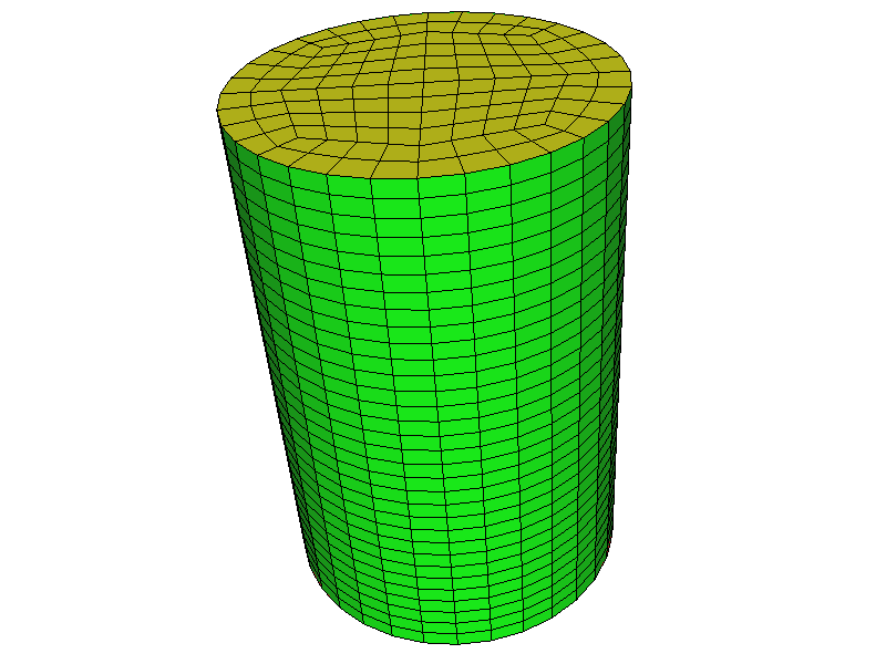
# mesh of a cylinder, base is a mesh of a disk, z belongs to [-1,1]
# we consider that the 2-D mesh contains only one reference
# (nb_ref_surf = nb_ref_volume = 1)
# therefore 2 will be the reference of lateral section and 3 of the
# top section
FileMesh = EXTRUDE 1 -1.0 1.0 disque.mesh AUTO \
1 2 3 \
1 1
Related topics :
Location :
AdditionalMesh
Syntax :
AdditionalMesh = nom_fichier
Actually, the syntax is the same as FileMesh. The aim of this keyword is to load additional meshes after the initial mesh. For almost all the simulations, these additional meshes won't be read... The initial aim of this entry was to deal with non-conformal meshes and load each part of the mesh separately, but non-conformal meshes are not currently handled by Montjoie .
Example :
# First, you specify the initial mesh
FileMesh = first.mesh

# then you can add as many meshes as you want
AdditionalMesh = second.mesh
AdditionalMesh = third.mesh
Location :
NbProcessorsPerMode
Syntax :
NbProcessorsPerMode = n
This entry is still experimental and should not be used.
Example :
NbProcessorsPerMode = 8
Location :
Harmonic/DistributedProblem.cxx
SaveSplitDomain
Syntax :
SaveSplitDomain = YES file_name
If you add this keyword, the partioning of the mesh is saved through the array Epart. The Epart array is an array that gives for each element the processor number. This array is saved in binary in the specified file.
Example :
# partitioning saved in the file Epart.dat
SaveSplitDomain = YES Epart.dat
Location :
Harmonic/DistributedProblem.cxx
SplitDomain
Syntax :
SplitDomain = type_partitioning
This entry specifies the partioning tool used to split the mesh into several sub-domains for execution on parallel architecture. The default partitioning is Metis, you have the following choices:
- Metis : Metis partioning
- Scotch : Scotch partioning (available if Montjoie has been compiled with Scotch)
- Concentric : the mesh is split in concentric layers
- User : the user provides directly the Epart array
- Layered : the user provides a mesh with different physical areas
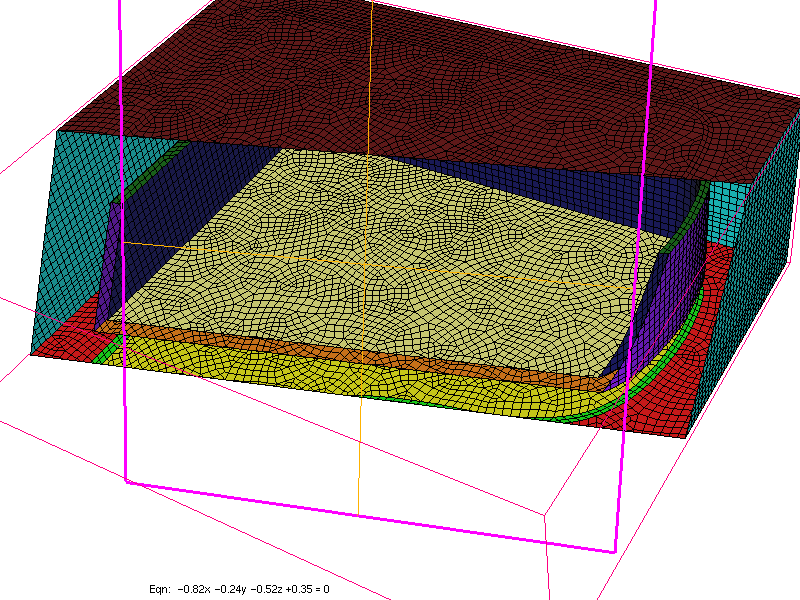
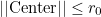
The Epart array is an array that gives for each element the processor number. If User partioning is selected, the user must provide a file containing this array of integers (in binary format). For concentric layers, the user provides a set of radii rn. All the elements whose center satisfy the condition :
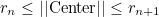
belong to the processor n+1. The processor 0 takes elements such that :
The last processor takes elements such that:
This partioning creates circular layers in 2-D, and spherical layers in 3-D.
Example :
# partitioning with Scotch
SplitDomain = Scotch

# user-partitioning
# the user provides the array epart in a binary file
SplitDomain = User file_with_epart.dat

# concentric partioning
# the user provides radii, and elements between r_n and r_{n+1}
# belong to processor n
# for two processors, you have to specify only one radius
SplitDomain = Concentric 1.5

# Layered partitioning
# each reference (Physical Volume in 3-D, Physical Surface in 2-D)
# belongs to a different processor
SplitDomain = Layered AUTO

# you can manually set the references for each processor
# for each processor, you write nb_ref ref0 ref1 ... ref_n
# In this example, processor 0 is associated with references 1 and 5
# processor 1 is associated with references 2, 4 and 6
SplitDomain = Layered 2  1 5   3   2 4 6
Location :
Harmonic/DistributedProblem.cxx
TypeMesh
Syntax :
TypeMesh = type
You can specify the type of elements to use in the case of regular meshes generated by the code as described in the description of the keyword FileMesh. This type is also used to determine if the original mesh is split into small elements to satisfy the requirements. In 2-D, you have the following types:
- TRI : the mesh contains only triangles. If the original mesh contains quadrilaterals, each quadrilateral is split into two triangles.
- QUAD : the mesh contains only quadrilaterals. If the original mesh contains triangles, each triangle is split into three quadrilaterals and each quadrangle is split into four quadrilaterals
In 3-D, you have the following types:
- TETRA : the mesh contains only tetrahedra. If the original contains other elements, they are split into tetrahedra.
- HEXA : the mesh contains only hexahedra. If the mesh is purely tetrahedral, each tetrahedra is split into four hexahedra.
- PYRAMID : the regular mesh contains only pyramids. No splitting is performed if the original mesh contains other elements.
- WEDGE : the regular mesh contains only wedges (triangular prisms). No splitting is performed if the original mesh contains other elements.
- HYBRID : the regular mesh contains pyramids and tetrahedra.
Below, we show some illustrations of regular meshes created by Montjoie
| |
|
The two types of regular meshes in 2-D (REGULAR) with specifying TypeMesh = TRI or TypeMesh = QUAD
| |
|
Several patterns for meshing an elementary cell (REGULAR).
Example :
# In 2-D, you can use triangular or quadrilateral mesh
TypeMesh = TRI
TypeMesh = QUAD

# In 3-D, more choices are available
# HYBRID corresponds to the case where each cube is made of 2 tets and
# 2 pyramids
TypeMesh = TETRA
TypeMesh = PYRAMID
TypeMesh = HYBRID
TypeMesh = WEDGE
TypeMesh = HEXA
Related topics :
Location :
Mesh/Mesh2D.cxx
Mesh/Mesh3D.cxx
MeshPath
Syntax :
MeshPath = directory
Often the meshes are always in the same directory. As a result, you can specify this directory, and the meshes will be searched inside this directory. The default directory is the current directory.
Example :
# You can use current directory and enter the relative path of the mesh in FileMesh
MeshPath = ./
FileMesh = MyDirectory/MyMeshes/cube.mesh

# Or you can separate the directory from the file
MeshPath = MyDirectory/MyMeshes/
FileMesh = cube.mesh
Location :
IrregularMesh
Syntax :
IrregularMesh = YES
IrregularMesh = NO
If you want bad quadrilateral/hexahedral meshes, you can insert this entry, and it will generate tetrahedral meshes split into hexahedra. In 2-D, the regular mesh will be made of triangles split into quadrilaterals. The default value is NO.
Example :
IrregularMesh = YES
Location :
SlightModificationOnRegularMesh
Syntax :
SlightModificationOnRegularMesh = YES
SlightModificationOnRegularMesh = RANDOM
This functionality is available in 3-D only and modifies the regular mesh (if FileMesh = REGULAR is present) such that there are non-affine elements. In order to generate non-affine elements, one vertex out of 2 (in each direction) is translated:
If YES is selected each odd vertex is translated with this same quantity. If RANDOM is selected, each odd vertex is vertex by this quantity multiplied by random numbers (between -1 and 1) for each component.
Example :
# non-affine elements with a fixed translation vector
SlightModificationOnRegularMesh = YES

# non-affine elements with a random translation
SlightModificationOnRegularMesh = RANDOM
Location :
RefinementVertex
Syntax :
RefinementVertex = x y level ratio
For 2-D meshes, you can ask a local refinement around the vertex of coordinates (x,y). level is the number of refinements performed, and ratio the quotient of coarse edge to fine edge. There is no local refinement applied by default.
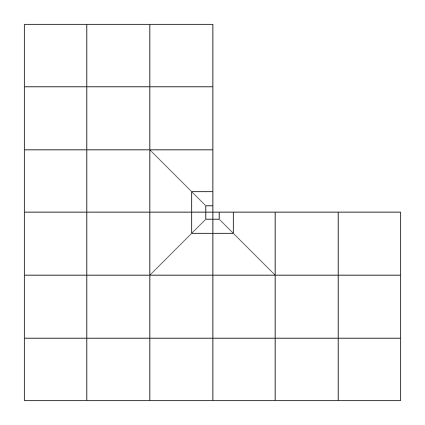 |
Local refinement around vertex (0, 0) with two levels and ratio equal to 3.0.
Example :
# around point (1,0), you locally refine 5 times with a ratio of 2.
RefinementVertex = 1 0 5 2.0
Location :
AddVertex
Syntax :
AddVertex = x y
For 2-D meshes, you can ask to create a new vertex. The mesh will be modified in order to include this vertex while being conformal. There can be triangles generated by the process.
Example :
# you want to create a new point (-2.5, 0.3)
AddVertex = -2.5 0.3

# then you can ask a local refinement around this vertex
RefinementVertex = -2.5 0.3  5  2.0
Location :
ThresholdMesh
Syntax :
ThresholdMesh = eps
You can specify a given threshold for 2-D (or 3-D points). The default value is 1e-10. If the distance between two points is below this threshold, they are assumed to be the same.
Example :
# depending on the characteristic length, you may modify the threshold for points of the mesh :
ThresholdMesh = 1e-12
Location :
TypeCurve
Syntax :
# curves in 2-D
# a circle of center (x0, y0) and radius r0
TypeCurve = ref1 ... refn CIRCLE x0 y0 r0
# an ellipse (of axis x and z)
TypeCurve = ref1 ... refn ELLIPSE x0 y0 a b
# a C1 spline
TypeCurve = ref1 ... refn SPLINE
# local spline (i.e. on each edge, we use a third order approximation
by using neighboring points, but this technique does not lead to a C1
curve)
TypeCurve = ref1 ... refn LOCAL_SPLINE


# curves in 3-D
# a sphere of center (x0, y0, z0, r0)
TypeCurve = ref1 ... refn SPHERE x0 y0 z0 r0
# a cylinder of radius r0 and axis (u0, v0, w0) and point (x0, y0, z0)
# belongs to the axi
TypeCurve = ref1 ... refn CYLINDER x0 y0 z0 u0 v0 w0  r0
# a cone of center (x0, y0, z0), of axis (u0, v0, w0) and angle teta
TypeCurve = ref1 ... refn CONE x0 y0 z0 u0 v0 w0 teta
You can specify curved surfaces, but a limited choice of curves is proposed. A more general solution is to directly provide a curved mesh (Gmsh produces curved meshes for instance). In 2-D, the use of splines is quite general, but provides only a third order approximation of the geometry. By default, no curves are present (elements are straight). In 2-D the following curves are proposed:
- CIRCLE x0 y0 radius: the curve is an arc of circle. The parameters can be given, if not the code will find the correct parameters automatically.
- ELLIPSE x0 y0 a b: the curve is an arc of ellipse.
- PEANUT x0 y0 a b c: the curve is a part of a peanut.
- SPLINE : the curve is approximated by cubic splines
- LOCAL_SPLINE : the curve is approximated by cubic polynomials (computed with only neighbor points).
In 3-D, the following curves are proposed:
- SPHERE x0 y0 z0 radius: the curved surface is a part of a sphere. The parameters can be given, if not the code will find the correct parameters automatically.
- CYLINDER x0 y0 z0 u0 v0 w0 radius: the curved surface is a part of a cylinder whose axis is directed along (u0, v0, w0) and (x0, y0, z0) is a point on the axis. The parameters can be given, if not the code will find the correct parameters automatically.
- CONE x0 y0 z0 u0 v0 w0 alpha: the curved surface is a part of a cone whose axis is directed along (u0, v0, w0) and (x0, y0, z0) is a point on the axis, alpha is the angle of the cone. The parameters can be given, if not the code will find the correct parameters automatically.
Example :
# If you don't specify the parameters of the circle, the
# code finds them automatically
TypeCurve = 1 CIRCLE

# For ellispes, you need to fill parameters ...
TypeCurve = 2 ELLIPSE 0.0 0.0  3.0 1.0

# For SPLINE, no bifurcation is allowed (a curve with two branches).
# It is allowed for LOCAL_SPLINE, but the result should be ugly ...
TypeCurve = 4 SPLINE


# For spheres, cylinders and cones, you don't need to specify parameters, they are automatically found by an optimization procedure
TypeCurve = 3 SPHERE
TypeCurve = 5 CYLINDER
TypeCurve = 6 CONE
Location :
MateriauDielec
Syntax :
MateriauDielec = ref ISOTROPE rho mu sigma
This entry is useful to specify physical properties of a media, such as dielectric permittivity epsilon and magnetic permeability mu for Maxwell's equations. Since it depends on the considered equation, we refer the reader to the sections devoted to each equation : Helmholtz, Maxwell, Aeroacoustics, Elastic. The default values are 1 (and 0 for damping indexes). Each index can be constant (e.g. 2.4, 0.5, etc) or variable. In order to specify a variable coefficient, we expect one of the following value :
- RANDOM : the index is given through its values on a regular grid. Fourth-order interpolation is performed to compute the values on quadrature points
- SINUS : the index is a product of sine functions
- MESH : the index is given on a mesh (different from the computational mesh), currently this functionality has been disabled
- SAME_MESH : the index is given on the same mesh as the computational mesh
- PERIODIC : it is similar to RANDOM, the index is periodized outside the bounding box
- QUASI_PERIODIC : it is similar to RANDOM, the index is periodized outside the bounding box (except on the center cell where the index is constant)
- RADIAL : the index is assumed to be radial (it depends only on r). In a file the user gives the radii and associated values of the index. Cubic spline interpolation is used to interpolate on quadrature points.
- USER : the index is given analytically by the user in the file UserSource.cxx (function ComputeVariableUserIndex). In that case, no interpolation is performed.
- VELOCITY : the index is equal to 1/c2 where c is the given constant
- SQUARE : the index is equal to c2 where c is the given constant
- ANGLE : the index is equal to teta π/180 where teta is the given constant
- any other value : the index is constant and equal to the given value
For each keyword, additional parameters are expected. As a result, each coefficient rho, mu, sigma indicated by the line :
MateriauDielec = ref ISOTROPE rho mu sigma
can be replaced by one of the following choice :
- constant_value
- ANGLE teta
- SQUARE c
- VELOCITY c
- USER offset amplitude coef_infinity
- RADIAL file_index
- RANDOM xmin xmax ymin ymax (zmin zmax) coefx coefy (coefz) offset amplitude file_index PRECISION coef_infinity
- PERIODIC xmin xmax ymin ymax (zmin zmax) coefx coefy (coefz) offset amplitude file_index PRECISION coef_infinity
- QUASI_PERIODIC xmin xmax ymin ymax (zmin zmax) coefx coefy (coefz) offset amplitude file_index PRECISION coef_infinity
- MESH mesh_file offset amplitude data_file order coef_infinity
- SAME_MESH mesh_file offset amplitude data_file order coef_infinity
- SINUS xmin xmax ymin ymax (zmin zmax) coefx coefy (coefz) offset amplitude kx ky (kz) coef_infinity
The fields inside parenthesis are needed in 3-D only. coef_infinity is needed when the inhomogeneous media encounters an absorbing boundary condition or PML layers, because they need the knowledge of the value of physical indices at infinity. All these parameters can lead to a lengthy line, usually we put the character '\' to separate each index. Another alternative is to use the keyword PhysicalMedia such that you specify each index on a separated line. Below we describe the different choices of varying media.
SINUS is used when you want to have a sinusoidal variation of coefficient on a bounding box [xmin, xmax] x [ymin, ymax]. Outside the bounding box, the coefficient will be equal to offset. The formula used for SINUS is :

MESH is used when you know the coefficient on a mesh. There will be problems if the mesh provided does not contain the mesh where the simulation is performed, that often occurs when curved boundaries are present. As a result, this functionality has been disabled. If you use the same mesh for the simulation and the definition of the coefficient, you have to write SAME_MESH since the interpolation is obvious and is not time consuming. In order to produce the data file, you have to start from an initial data file such as:
TypeElement = QUADRANGLE_LOBATTO
TypeEquation = TIME_REISSNER_MINDLIN

# path where the meshes are stored
MeshPath = ./

# frequency of the temporal source
# Frequency = a b means that the pulsation omega = 2*pi*a + b
Frequency = 5.0 0.0

# file where the mesh is stored
FileMesh = plaque.mesh

# In practice all the triangles are split into quadrilaterals
# so you have to write this line
TypeMesh = QUAD

# order of space approximation
OrderDiscretization = 4

# other fields are not very important for the next step
The only requirement in this data file is that all lines related to the mesh are present (such as RefinementVertex, TypeMesh, etc) and the order of discretization. Nodal points on the resulting mesh are generated by write_nodal. If write_nodal has not been compiled, you can compile it by writing :
make write_nodal
Nodal points (that are written in the file nodal_points.dat) and the resulting mesh (written in the file test.mesh) are generated by executing write_nodal:
./write_nodal.x time_carre_plate.ini
The second argument is the name of the data file. A third optional argument is the order of approximation. If this argument is provided, eg.:
./write_nodal.x time_carre_plate.ini 10
It will ignore the value given in the data file and use this value (here 10). It can be useful if you want to use different orders of approximation, one for the finite element computation and one for the definition of the index. It is advised to copy the resulting mesh in another file :
cp test.mesh test_plaque.mesh
Then, you can implement the computation of the index from coordinates. You can start from the file src/Program/Test/write_index.cc, copy it in another file and write the implementation of your index. write_index.cc evaluates the index as a continuous index. You can provide piecewise continuous indexes, with continuous index for each reference of the mesh. If you want to specify a piecewise continuous index, you can start from the file src/Program/Test/write_index_plaque.cc and modify the function ComputeIndex:
// x, y : coordinates of the 2-D point where the index must be evaluated
// ref : reference of the element where the point is
// n : index number
// delta : value of the index n at this point
void ComputeIndex(const Real_wp& x, const Real_wp& y, int ref, int n, Complexe& delta)
{
  switch (ref)
    {
    case 1: delta = 0.002*exp(-(x*x+y*y)); break;
    case 2 : delta = 0.005; break;
    case 5 : delta = 0.01*exp(-0.3*x*x); break;
    case 6 : delta = 0.007*exp(-0.5*y*y); break;
    }
}
The file containing the values of the index is then generated by compiling and executing the file you have modified :
./write.x nodal_points.dat test_plaque.mesh index.don
You can specify several file names after index.don if there are several indexes to evaluate. In that case, n will refer to the index number. Once the index file has been generated, you can fill your line in the data file
# SAME_MESH maillage offset amplitude file_index order coef_infinity
MateriauDielec = 1 ISOTROPE SAME_MESH test_plaque.mesh 0.0 1.0 index.don 4 1.0
MateriauDielec = 2 ISOTROPE SAME_MESH test_plaque.mesh 0.0 1.0 index.don 4 1.0
The order provided is the order used to generate the file nodal_points.dat. It can be different from the order used in the simulation. Here you have to repeat the same line for each reference. The final value of rho will be equal to :
offset + amplitude * delta
where delta corresponds to values contained in the file index.don.
RANDOM is used when you want to have a variation of coefficient specified by a file on a box [xmin, xmax] x [ymin, ymax] (x [zmin, zmax] in 3-D). Outside the box, the coefficient will be equal to offset. The formula used for RANDOM is :

The function h(x,y) is computed with fourth-order interpolation of values of h on a regular grid (these values are directly given in a file). You can write these values in binary format from a dense matrix nu with the Matlab functions write_full_?.m (contained in the folder MATLAB, with the Blas convention c, d, s, z for complex float, double, float, and complex double). You can also write the indices with Python, for example if you execute the following lines:
X = linspace(-5.0, 5.0, 400);
Y = linspace(-3.0, 3.0, 240);
[XI, YI] = meshgrid(X, Y);
rho = cos(0.5*pi*XI)*sin(pi*YI);
write_full("../rho_var.don", transpose(rho));
The transpose is here due to the meshgrid function and is inherent to 2-D fields. In Matlab write_full has to be replaced by write_full_d in this case (double precision). In Python, write_full handles both real and complex data, a third argument optional is used to switch to single precision :
write_full("../rho_var.don", transpose(rho), False);
In this last case, rho_var.don is written in single precision. In the data file, you have to specify the type of data (FLOAT, DOUBLE, COMPLEX or COMPLEX_DBLE). For example, you can write
Example :
# MateriauDielec = 1 ISOTROPE RANDOM xmin xmax ymin ymax coefx coefy offset amplitude file_index PRECISION coef_infinity
# the two last values here are mu and sigma
MateriauDielec = 1 ISOTROPE RANDOM -2 2 -2 2 0 0 0.5 0.1 rho_var.don DOUBLE 1.0 \
                                   2.5 0.5
PERIODIC uses the same formula as for RANDOM. The difference is that the point x is translated into the specified bounding box before applying the formula. By construction, the index will be periodic with a period given by the bounding box.
QUASI_PERIODIC is almost equivalent to PERIODIC. The only difference is that if the point is in the central cell (not translated), the index will be set to the given offset. As a result the physical index is uniform in the central cell, and periodic in all other cells.
USER will use directly the function ComputeVariableUserIndex to compute the variable index. In this function, the index number refers to a given index (0 for rho, 1 for mu, 2 for sigma, etc) and the component number to a component of the index (for vectors or tensors). In that case, the user must modify the file Source/UserSource.cxx to enter the desired expression, recompile the code and launch it. The data file will have a line of the type
Example :
# if you want a variable rho and mu
# USER offset amplitude coef_infinity for each index
MateriauDielec = 1 ISOTROPE USER 0.5 1.0 1.0 USER 0.0 2.0 1.0
RADIAL specify an index that depends on the norm of x (i.e. the radius). The values of the index are given in a text file with two columns:
r0 index0
r1 index1
r2 index2
The first column contains the different radii, the second column the associated values. A cubic spline is contructed from this data to interpolate the index on any point.
If you have a print level greater or equal to 7, and if you are running the code in sequential, varying indexes will be written in files :
rho_ref1_G0_U0.dat
rho_ref1_G1_U0.dat
mu_ref1_G0_U0.dat
rho_ref2_G0_U0.dat
...
The file names begin with the name of the physical index (rho, sigma, mu, epsilon, etc) then the reference number follows, then the grid number and finally the component of the index.
Location :
Harmonic/VarProblemBase.cxx
Elliptic/PhysicalProperty.cxx
PhysicalMedia
Syntax :
PhysicalMedia = name_media ref ISOTROPE parameters
This entry is useful to specify physical properties of a media. The media can be uniform, in that case parameters will contain the numerical values of the media. It can also be non-uniform, and each component of the physical media has to be specified as detailed in MateriauDielec. The keyword PhysicalMedia is more convenient, because you specify a different kind of anisotropy for each media whereas the type of anisotropy is common in MateriauDielec. The names of physical media are detailed in the section devoted to the desired equation.
Example :
# For Maxwell's equations, there are three physical indexes : epsilon, mu, sigma
# here we specify different anisotropy for the three indexes (which are matrices)
PhysicalMedia = epsilon 1 ISOTROPE 2.0
PhysicalMedia = mu 1 ORTHOTROPE 1.0 1.5 1.8
PhysicalMedia = sigma 1 ANISOTROPE 0.1 0.02 0.01  0.2 0.005  0.3
ExactIntegration
Syntax :
ExactIntegration = YES
ExactIntegration = NO
ExactIntegration = YES order
ExactIntegration = NO order
For discontinuous Galerkin formulation, if you say YES, you will use an unsplit formulation, which will be probably stable if integrals are exactly computed (i.e. you are using Gauss points), if you say NO, a split formulation will be used, slower but stable for approximate integration. Details are avaible in the paper of N.Castel, G. Cohen and M. Duruflé. This value is important only for aeroacoustics and default value is YES. The optional parameter order is the over-integration that can be used.
Example :
ExactIntegration = NO
Location :
Harmonic/VarProblemBase.cxx
Elliptic/PhysicalProperty.cxx
MixedFormulation
Syntax :
MixedFormulation = YES_OR_NO
If the user specifies a mixed formulation, the second-order equation such as Helmholtz equation :
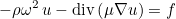
is transformed in a first-order system, e.g :
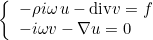
This kind of transformation is implemented for Helmholtz equation, Maxwell's equations and elastodynamics. When continuous (or edge elements for Maxwell's equations) finite elements are used to solve one of these equations, the additional unknown v is chosen discontinuous. The advantage of this first-order system is that it is well adapted to time-domain simulations (with the adjunction of PML layers). This mixed formulation is automatically chosen if the selected time scheme is a scheme adapted to first-order formulation (such as Runge-Kutta schemes). For time-harmonic simulations, there is no interest in considering this mixed formulation. As a result, the mixed formulation is not chosen by default, you can force to use it by inserting this line in the data file. This formulation is interesting for the computation of eigenmodes, since the eigenvalue problem is linear with respect to omega even with PML or first-order absorbing boundary condition.
Example :
MixedFormulation = YES
Location :
PenalizationDG
Syntax :
PenalizationDG = alpha delta
For Discontinuous Galerkin formulation and linear problems, additional stabilizing terms need to be incorporated into the discontinuous Galerkin formulation (we can call them penalty terms as well). This is somehow equivalent to choose upwind fluxes instead of centered fluxes, which correspond to take alpha and delta equal to 0. Default choice is upwind fluxes, negative values provide more stability (positive values are instable).
Example :
# Classical choice of parameters -1, -1
PenalizationDG = -1.0 -1.0

# upwind fluxes :
PenalizationDG = Upwind

# centered fluxes :
PenalizationDG = 0.0 0.0
Location :
CoefficientPenalization
Syntax :
CoefficientPenalization = AUTO
For Discontinuous Galerkin formulation and linear problems, additional stabilizing terms need to be incorporated into the discontinuous Galerkin formulation (we can call them penalty terms as well). For SIPG (Symmetric Interior Penalty Galerkin), the coefficient depends on the order and the mesh size as:

By default, this coefficient is chosen and multiplied by the first coefficient given in PenalizationDG. If you do not want to start from this value, you can put this line with MANUAL (instead of AUTO) and the coefficient is then directly given in PenalizationDG.
Example :
# if you put auto, the penalization term is equal to
#  beta \int_{\partial K} [u] [v] (for Helmholtz equation)
# beta will be equal to 2.0 * alpha where alpha = r(r+1) / h
# usually this value works pretty well for any kind of mesh, you can
# modify the 2.0 in Penalization DG (the negative sign is mandatory)
CoefficientPenalization = AUTO
PenalizationDG = -2.0 0.0

# if you want to set beta directly :
CoefficientPenalization = MANUAL
PenalizationDG = -100.0 0.0
Location :
PointDirichlet
Syntax :
PointDirichlet = x0 y0 z0
You can specify dirichlet conditions on vertices for continuous finite elements by entering the coordinates of the vertices. When it is used to recover uniqueness of the solution for a Poisson equation with only Neumann boundary conditions, it doesn't work as nicely as expected since the point where Dirichlet condition is enforced is obvious to detect when you look at the solution. There is no default value.
Example :
# in 3-D :
PointDirichlet = 1.0 -2.0 3.0

# you can add as many lines you want
# each line will appends a new Dirichlet node
PointDirichlet = 0.0 5.0 2.4
Location :
Harmonic/BoundaryConditionHarmonic.cxx
OrderAbsorbingBoundaryCondition
Syntax :
OrderAbsorbingBoundaryCondition = order
When you write ConditionReference = 1 ABSORBING, an absorbing boundary condition is set on edges of reference 1. By default, this condition is a first order absorbing boundary condition. For Helmholtz equation only, some high order absorbing boundary conditions are available.
Example :
OrderAbsorbingBoundaryCondition = 1

# For Helmholtz equation, 2 is the classical second-order ABC with Laplace-Beltrami operator (Joly-Vacus)
OrderAbsorbingBoundaryCondition = 2

# other boundary conditions has been developed by Chabassier, Bergot, Barucq
OrderAbsorbingBoundaryCondition = 2 GRAZING

# PARAMETERS gamma theta zeta
OrderAbsorbingBoundaryCondition = 2 PARAMETERS 0.25 0.5 0.5

# PARAMETERS gamma theta zeta GRAZING
OrderAbsorbingBoundaryCondition = 2 PARAMETERS 0.25 0.5 0.5 GRAZING
Location :
Harmonic/BoundaryConditionHarmonic.cxx
ModifiedImpedance
Syntax :
ModifiedImpedance = CURVE
ModifiedImpedance = coef
For first-order absorbing boundary condition and Helmholtz equation, you can multiply the default impedance value (-i omega sqrt(rho mu) ) by a coefficient. This can be useful for circular boundaries, where the modification of this impedance will reduce reflection. For curved boundary, you can write the keyword CURVE, such that the usual factor h is added (h is the mean curvature).
Example :
# first-order absorbing boundary condition
OrderAbsorbingBoundaryCondition = 1

# usually if the boundary is curved, we have du/dn = (ik + h) u
# where h is the mean curvature (k1+k2)/2
# if you want to take into account this term, you put CURVE
ModifiedImpedance = CURVE

# another possibility is to set directly a coef such that
# du/dn = ik coef u
# you write the coefficient coef below:
ModifiedImpedance = (1.002,0.002)
Location :
Harmonic/BoundaryConditionHarmonic.cxx
OrderHighConductivityBoundaryCondition
Syntax :
OrderHighConductivityBoundaryCondition = order
Objects with a high conductivity can be replaced by an equivalent boundary condition. Order 0 is the classical perfectly conducting boundary condition. Order 1, 2 and 3 are implemented and provide more accurate results. The implementation is achieved only for Helmholtz equation and axisymmetric Maxwell equations. Default value is set to 0.
Example :
OrderHighConductivityBoundaryCondition = 3
Location :
Harmonic/BoundaryConditionHarmonic.cxx
Exit_IfNo_BoundaryCondition
Syntax :
Exit_IfNo_BoundaryCondition = YES
Exit_IfNo_BoundaryCondition = NO
When an isolated boundary (belonging to only one element) is found, and there is no associated boundary condition, the code will stop the simulation. If you want to continue the simulation, you have to insert this entry.
Example :
Exit_IfNo_BoundaryCondition = NO
Location :
ConditionReference
Syntax :
ConditionReference = n1 n2 ... nk DIRICHLET
ConditionReference = n1 n2 ... nk NEUMANN
ConditionReference = n1 n2 ... nk ABSORBING
ConditionReference = n1 n2 ... nk HIGH_CONDUCTIVITY epsilon
ConditionReference = n1 n2 ... nk IMPEDANCE lambda
ConditionReference = n1 n2 PERIODICITY
Each entry of this type has to be inserted for each considered boundary condition. Dirichlet, Neumann, absorbing, impedance or periodic boundary conditions are classical and implemented for all the equations solved by Montjoie. High conductivity boundary condition is only available for Helmholtz and time-harmonic Maxwell's equations. For each condition, you can specify an arbitrary number of references (the integers n1, n2, ..., nk). These reference numbers are the physical line numbers defined in the mesh (for Gmsh). For periodic conditions, two and only two references are required, the reference of the two parallel hyperplanes.
Example :
# accepted types : DIRICHLET, SUPPORTED, NEUMANN, ABSORBING, HIGH_CONDUCTIVITY, IMPEDANCE
# SUPPORTED is used for Reissner-Mindlin or elastodynamics
# such that you specify Dirichlet condition for some components
# and Neumann condition for other components
ConditionReference = 1 2 3 DIRICHLET
ConditionReference = 4 NEUMANN
ConditionReference = 5 6 ABSORBING
ConditionReference = 5 6 HIGH_CONDUCTIVITY 0.1
ConditionReference = 7 8 9 IMPEDANCE 2.5

# For periodic conditions, you can choose among
# PERIODICITY, PERIODIC_X, PERIODIC_Y, PERIODIC_Z, CYCLIC
# PERIODIC_X, PERIODIC_Y, PERIODIC_Z, CYCLIC will induce that
# Fourier series of the source are computed such that
# the user gives only a generating part of the geometry
ConditionReference = 10 13 PERIODICITY
Location :
Harmonic/BoundaryConditionHarmonic.cxx
ForceDirichletSymmetry
Syntax :
ForceDirichletSymmetry = YES
By writing YES, the user asks to treat Dirichlet condition in the same way for symmetric or unsymmetric matrices. By default, if the matrix is unsymmetric, rows associated with Dirichlet dofs are replaced by zeros with one on the diagonal. This operation "unsymmetrizes" the matrix. If the matrix is symmetric, rows and columns associated with Dirichlet dofs are erased except one on the diagonal. Columns are stored such that the right-hand side is modified with a hetereogeneous Dirichlet condition. By writing YES, this treatment (usually performed for symmetric matrices) is performed whatever is the type of the finite element matrix. The solution should the same, it may improve the condition number of the matrix.
Example :
ForceDirichletSymmetry = YES
Location :
Harmonic/BoundaryConditionHarmonic.cxx
DirichletCoefMatrix
Syntax :
DirichletCoefMatrix = alpha
By default, if the matrix is unsymmetric, rows associated with Dirichlet dofs are replaced by zeros with one on the diagonal. Instead of one, the user can provide its own coefficient.
Example :
DirichletCoefMatrix = 1e5
Location :
Harmonic/BoundaryConditionHarmonic.cxx
StorageModes
Syntax :
StorageModes = YES
When a cyclic condition is imposed (or PERIODIC_X, PERIODIC_Y, PERIODIC_Z), the solution is computed through its Fourier series. Each mode can be stored, and the final solution is obtained by applying a FFT. However, the user can ask that the modes are not stored (to reduce the memory usage), in that case the solution is incremented (FFT can no longer be used).
Example :
# you can write YES or NO
StorageModes = YES
Location :
Harmonic/BoundaryConditionHarmonic.cxx
NbModesPeriodic
Syntax :
NbModesPeriodic = nx ny nz
When periodic conditions are imposed (PERIODIC_X, PERIODIC_Y and/or PERIODIC_Z), the solution is computed through its Fourier series. You need to give the number of Fourier modes along each direction. For CYCLIC, it is not needed to specifiy this number, since the code will detect automatically the angle between the two cyclic boundaries and deduce the number of modes.
Example :
# if you have periodicity in y and z for example :
ConditionReference = 1 3 PERIODIC_Y
ConditionReference = 2 4 PERIODIC_Z

# Number of modes for each direction (here one mode for x)
NbModesPeriodic = 1 8 16
Location :
Harmonic/BoundaryConditionHarmonic.cxx
TransverseDampingPML
Syntax :
TransverseDampingPML = ratio
You can add a damping in the transverse direction (in y if the PML is in x). By doing that, the PML is no longer PML, but it can eliminate instabilities (e.g. in elastodynamics).
Example :
# this ratio should be small compared to 1
TransverseDampingPML = 0.01
Location :
Harmonic/BoundaryConditionHarmonic.cxx
DampingPML
Syntax :
DampingPML = alpha
DampingPML = fct parameters
You can increase damping coefficient inside PML in order to reduce the reflection on the outside boundary. Default value is set to 1.0, for which a reflection of 0.1 % should be observed for a thickness of one wavelength. This keyword can also be used to specify a different damping function (different from the usual parabolic function). For a parabolic damping we consider the following expression
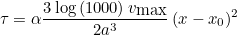
where a is the thickness of the PML, vmax is the maximal velocity in the PMLs and x0 the starting position of PML. The coefficient alpha corresponds to the value given in DampingPML. For a constant function, we consider :
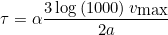
SHIFTED_PARABOLE corresponds to the following expression
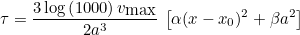
Example :
# 2.0 should provide an error of 1e-6
DampingPML = 2.0

# if you want to define other damping functions
# for example a constant damping :
# available choices are CONSTANT, PARABOLE and SHIFTED_PARABOLE
DampingPML = CONSTANT 1.0

# you can indicate a linear profile
DampingPML = LINEAR 1.0

# for shifted parabole, you specify a and b (in the expression a x^2 + b)
DampingPML = SHIFTED_PARABOLE 2.0 0.5
Location :
Harmonic/BoundaryConditionHarmonic.cxx
AddPML
Syntax :
AddPML = YES axis thickness nb_layers
AddPML = ref type_pml thickness nb_layers
PML layers are not generated during the meshing phase, they are directly added by Montjoie thanks to that entry. You ask the code to add PML layers around the provided mesh. You have to specify the thickness of PML layers (often we take one wavelength), and the number of layers (e.g. one layer is usual with a Q7 approximation). For this last parameter, you can enter AUTO so that the number of layers is automatically computing depending on the thickness and the mesh step. the parameter "axis" is a combination of X, Y, Z, X+, X-, Y+, Y-, Z-, Z+ such that you can add PML layers in any direction you want. By default, no PML layers are added.
Example :
# If you want PML in X and Y, of thickness 1, number of layers is automatically chosen
AddPML = YES XY 1.0 AUTO

# If you want only PML in the right side, and bottom side :
AddPML = YES X+Y- 1.0 2

# If you want PML only for z > 0
AddPML = YES Z+ 2.0 3

# for radial PML : PML_R
AddPML = YES PML_R 1.0 AUTO

# for a mix of radial and cartesian PML, we
# extrude PML from a reference
AddPML = 2 PML_R 0.4 2
Location :
EigenvalueTolerance
Syntax :
EigenvalueTolerance = tolerance
You can specify here the stopping criterion used for the determination of eigenvalues. The default value is 1e-6.
Example :
EigenvalueTolerance = 1e-6
Location :
Solver/EigenvaluesHarmonic.cxx
EigenvalueMaxNumberIterations
Syntax :
EigenvalueMaxNumberIterations = nb_iter
You can specify here the maximum number of iterations for the eigenvalue solver. The default value is 1000.
Example :
EigenvalueMaxNumberIterations = 1000
Location :
Solver/EigenvaluesHarmonic.cxx
UseCholeskyForEigenvalue
Syntax :
UseCholeskyForEigenvalue = YES
The Cholesky factorization of the mass matrix is computed such that the generalized eigenvalue problem

is transformed into a standard eigenvalue problem:
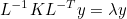
where L is the Cholesky factor of the mass matrix M.
Example :
UseCholeskyForEigenvalue = YES
Location :
Solver/EigenvaluesHarmonic.cxx
EigenvalueSolver
Syntax :
EigenvalueSolver = name
You can choose the solver to use (between Arpack, Feast or Slepc). The default solver is Arpack.
Example :
// if you want to choose Slepc
EigenvalueSolver = Slepc
Location :
Solver/EigenvaluesHarmonic.cxx
FileEigenvalue
Syntax :
FileEigenvalue = file_name
You can specify here the file where the eigenpulsations are written. By default, the eigenpulsations are written in the file Omega.dat. They are written in binary format (loadable with load1D in Python).
Example :
FileEigenvalue = Omega.dat
Location :
Solver/EigenvaluesHarmonic.cxx
Eigenvalue
Syntax :
Eigenvalue = YES mode shift nb_eigenvalues
You can ask the computation of eigenvalues of the following generalized eigenvalue problem:

where K is the stiffness matrix, M the mass matrix. For Laplace equation (and continuous finite elements), these matrices are given as:
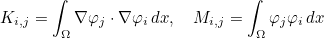
This eigenvalue problem is solved by calling an eigenvalue solver interfaced in Seldon (i.e. Arpack, Anasazi or Feast). The different modes of eigenvalues computation are the following:
- REGULAR : regular mode, the largest eigenvalues of M-1 K are searched. This modes does not involve a factorization of a linear system.
- SHIFTED : shifted mode, the largest eigenvalues of
 are computed in order to obtain eigenvalues close to the shift
sigma.
are computed in order to obtain eigenvalues close to the shift
sigma. - COMPLEX_SHIFT : complex-shifted mode, the largest eigenvalues of
 where the shift sigma is complex, only the imaginary part of the
factorized matrix is used here (whereas the real part is used for
SHIFTED).
where the shift sigma is complex, only the imaginary part of the
factorized matrix is used here (whereas the real part is used for
SHIFTED). - BUCKLING : Buckling mode, the largest eigenvalues of
 are computed in order to obtain eigenvalues close to the shift sigma.
- CAYLEY : Cayley mode, the largest eigenvalues of
 are computed in order to obtain eigenvalues close to the shift sigma.
- INVERT : this mode consists of transforming a generalized eigenvalue problem into a standard eigenvalue problem by solving mass matrix.
REGULAR mode is usually to avoid since it requires a lot of iterations in order to have all the needed eigenvalues. Therefore, for mass lumped elements, we advise to use SHIFTED, and for other elements, CAYLEY or INVERT mode can be used. shift is the frequency around which you want to know a given number of eigenvalues. shift can be equal to the following values:
- LARGE : largest eigenvalues are searched
- SMALL : smallest eigenvalues are searched
- COMPLEX : clustered eigenvalues are searched close to a complex shift
- shift : clustered eigenvalues are searched close to the given shift
Example :
# if you want 20 eigenvalues near frequency 0.5 for mass lumped elements
Eigenvalue = YES SHIFTED 0.5 20

# for 10 largest eigenvalues:
Eigenvalue = YES REGULAR LARGE 10

# for a real matrix and complex shift
Eigenvalue = YES COMPLEX_SHIFT COMPLEX 0.0 2.0 30
Location :
Solver/EigenvaluesHarmonic.cxx
Smoother
Syntax :
Smoother = type_smoother param_smoother
In this field, you specify the smoother used in multigrid preconditioning. Classical smoothers are available (JACOBI, BLOCK_JACOBI, SSOR), some equations can require a specific smoother like Maxwell's equations. The default smoother is Jacobi.
Example :
# Damped Jacobi with omega = 0.5
Smoother = JACOBI 0.5
# you can ask 2 iterations of Jacobi
Smoother = JACOBI 0.5 2

# similar for Block-Jacobi or Sor
Smoother = BLOCK_JACOBI 0.5
Smoother = SSOR 1.0
Location :
DampingParameters
Syntax :
DampingParameters = alpha delta
In this field, you specify the coefficient alpha used as damping for time-harmonic equations. delta is used in multigrid preconditioning if you want to decrease frequency on coarser grids. Default value of delta is 1. Default value of alpha is 1 for real problems and (1,0.5) for complex problems (advised value).
Example :
# example where the frequency will be multiplied by 0.7 for each coarser level
DampingParameters = (1.0,0.5) 0.7
Location :
DirectSolver
Syntax :
DirectSolver = MUMPS
DirectSolver = ILUT threshold type_ilu level_fill droptol permtol alpha_ilu
In this field, you specify the direct solver used by the coarsest level in multigrid preconditioning. Usually, you have to choose between a complete factorization (using Mumps for instance) or an incomplete factorization. Incomplete factorization can lead to a substantial gain in storage. The default value is MUMPS. threshold is the value above which all the values of the initial matrix are removed (in absolute value), droptol is the threshold used by incomplete factorization (in relative value).
Example :
# for a complete factorization
DirectSolver = MUMPS

# for an incomplete factorization with epsilon = 0.01 (common threshold)
DirectSolver = ILUT 1e-5 0 100000 1e-2 0.1 1
Location :
NumberMaxIterations
Syntax :
NumberMaxIterations = nb_max_iter restart
You can specify here the maximum number of iterations allowed for the iterative solution of finite element matrix, and the restart parameter (used by some Krylov solvers like GMRES and GCR). Default values are 1000 iterations allowed and a restart parameter equal to 10.
Example :
NumberMaxIterations = 1000 10
Location :
Tolerance
Syntax :
Tolerance = tolerance
You can specify here the stopping criterion used for the iterative solution of finite element matrix. The default value is 1e-6.
Example :
Tolerance = 1e-6
Location :
TypeResolution
Syntax :
TypeResolution = type_solver type_precond param_precond
You can specify here the iterative solver to use, preconditioning technique and optional parameters related to the preconditioner. In the table below, we present an exhaustive list of iterative solvers. We specify if the solver is able to solve symmetric complex, hermitian or unsymmetric matrices (all the solvers are of course able to solve symmetric real linear systems). Besides, some algorithms need the matrix-vector product with the transpose matrix. In the data file the name of the solver is written in capital letters.
| Name of the solver | Symmetric complex | Hermitian | Unsymmetric | Transpose matrix |
| BiCg | CoCg | Cg | Yes | Yes |
| BiCgcr | Yes | No | No | No |
| BiCgStab | Yes | Yes | Yes | No |
| BiCgStabl | Yes | Yes | Yes | No |
| Cg | No | Yes | No | No |
| Cgne | Yes | Yes | Yes | Yes |
| Cgs | Yes | No | Yes | No |
| CoCg | Yes | No | No | No |
| Gcr | Yes | Yes | Yes | No |
| Gmres | Yes | Yes | Yes | No |
| Lsqr | Yes | No | No | No |
| MinRes | Yes | No | No | No |
| QCgs | Yes | No | Yes | No |
| Qmr | Qmr_Sym | Yes | Yes | Yes |
| Qmr_Sym | Yes | No | No | No |
| Symmlq | Yes | No | No | No |
| TfQmr | Yes | Yes | Yes | No |
In this table, gray cells indicate which solver should be preferred for a symmetric or hermitian matrix. For example, if the matrix is symmetric, it is better to use CoCg instead of BiCg in order to save memory usage. Several preconditioning techniques are available (parameters are given in italic) :
- IDENTITY : the preconditioning is the identity matrix. If selected, the iterative algorithm will be performed without preconditioning.
- JACOBI omega nb_iter : the precondioning is damped Jacobi solver, omega is the relaxation parameter, nb_iter (optional parameter equal to 1) is the number of iterations
- BLOCK_JACOBI size_block omega nb_iter : the precondioning is damped block-Jacobi solver. size_block is the size of blocks (dofs that are close are gathered), omega is the relaxation parameter, nb_iter (optional parameter equal to 1) is the number of iterations
- SOR omega nb_iter : the preconditioning is S.O.R (Successive Over-Relaxations). omega is the relaxation parameter, nb_iter (optional parameter equal to 1) is the number of iterations
- SSOR omega nb_iter : the preconditioning is S.S.O.R (Symmetric Successive Over-Relaxations). omega is the relaxation parameter, nb_iter (optional parameter equal to 1) the number of iterations.
- ILUT type_facto lvl droptol pivot diag_coef : the preconditioning is Incomplete Factorization with threshold (ILUT). type_facto is equal to ILU_0, ILU_D, ILU_K or ILUT_K. lvl is the level k used by ILU(k) method. droptol is the dropping threshold, pivot the pivot threshold, diag_coef is used in ILU_D.
- DIRECT : the preconditioning is a direct solver.
- LOW_ORDER : the preconditioning is a direct solver for a finite element matrix constructed with first order and a subdivided mesh
- MULTIGRID nb_cycles rmin nb_smooth_iter: the preconditioning is an iteration of a multigrid solution. nb_cycles is the number of cycles (1 for a V-cycle, 2 for a W-cycle). rmin is the minimal order for which a direct solver will be used. If the coarse order is less or equal to this order, a direct solver is used. nb_smooth_iter is the number of smoothing iterations.
- SUBDOMAIN : the preconditioning is a basic subdomain preconditioning, each subdomain is associated with a processor.
Other preconditionings may be implemented for each specific solved equation. We have listed only preconditionings common for all equations.
Example :
# By default one iteration of Jacobi = diagonal preconditioning
TypeResolution = COCG JACOBI 1.0
# You can select more iterations (JACOBI omega nb_iter)
TypeResolution = COCG JACOBI 0.5 4
# or use Block-Jacobi algorithm (BLOCK_JACOBI size_block omega nb_iter)
TypeResolution = QMR_SYM BLOCK_JACOBI 10 0.5 1

# By default one iteration of SOR (SOR omega)
TypeResolution = BICGCR SOR 1.0
# You can select more iterations (SOR omega nb_iter)
TypeResolution = BICGCR SOR 1.5 4
# You can select more iterations or Symmetric SOR
TypeResolution = BICGCR SSOR 0.5 2

# Incomplete Factorization with threshold
# (ILUT threshold 0 max_elt droptol permtol alpha)
# max_elt is the maximum number of entries on a single row
# threshold is the value below which entries of original matrix are
# removed. droptol is the actual threshold used by incomplete factorization.
TypeResolution = GMRES ILUT 1e-5 0 100000 1e-2 0.1 1

# preconditioning by low-order elements (ok for interpolatory basis)
TypeResolution = BICGSTAB LOW_ORDER

# p-multigrid preconditioning (MULTIGRID gamma pmin nb_iter)
# gamma = 1 -> V-cycle, 2 -> W-cycle
# pmin is the minimal order used when decreasing order for coarse meshes
TypeResolution = QMR MULTIGRID 2 2 1
Location :
Solver/SolveSystem.cxx
Solver/Preconditioner.cxx
TypeSolver
Syntax :
TypeSolver = AUTO
TypeSolver = DIRECT
TypeSolver = ITERATIVE
TypeSolver = MULTIGRID
TypeSolver = ILUT
This field overrides the field TypeResolution, i.e. this last field won't be taken into account if you have defined TypeSolver in another part of the datafile. The aim of this field is to simplify how the user selects the solver he wants to use, because TypeResolution is more complex to fill. AUTO will select the "best" linear solver known for this problem, well it is not yet correctly implemented. DIRECT will select a direct solver, Mumps if available. ITERATIVE will select an iterative solver compatible with the type of matrix but without preconditioning, while MULTIGRID will use a multigrid preconditioning with ad hoc parameters. ILUT proposes an incomplete factorization as preconditioning.
Example :
TypeSolver = AUTO
Related topics :
Location :
PivotThreshold
Syntax :
PivotThreshold = eps
This field is used if you want to change the threshold to use for partial pivoting in the direct solver.
Example :
PivotThreshold = 1e-3
Location :
NbThreadsPerNode
Syntax :
NbThreadsPerNode = n
This field is used if you want to change the number of threads that will be launched (usually during numerical factorization of the finite element matrix) for each MPI process.
Example :
NbThreadsPerNode = 8
Location :
EstimationConditionNumber
Syntax :
EstimationConditionNumber = YES nb_iter
If you are using a direct solver, you can estimate the condition number of the finite element matrix. We use the formula lambda_max/lambda_min even if the matrix is not symmetric. The estimate of extrema eigenvalues is achieved by using a power iteration method on the matrix and its factorization.
Example :
EstimationConditionNumber = YES 20
Location :
Solver/SolveHarmonic.cxxStaticCondensation
Syntax :
StaticCondensation = YES
If you are using a direct solver, you can decrease the required storage by performing a static condensation (internal degrees of freedom are eliminated). This is particularly efficient for higher method and in 2-D.
Example :
StaticCondensation = YES
Location :
ScalingMatrix
Syntax :
ScalingMatrix = YES
Before the factorization (or the iterative solution), the finite element matrix can be scaled if this field is set to YES. The default value is NO, no scaling is performed if not asked. It may improve the convergence and accuracy (due to round-off errors).
Example :
ScalingMatrix = YES
Location :
MumpsMemoryCoefficient
Syntax :
MumpsMemoryCoefficient = coef_init coef_max inc_coef
You can change the parameters used in Mumps to factorize the finite element matrix. coef_init is the initial ratio used to store the factorization (compared to the estimate). A value of 1.0 means that you will use the memory as estimated. Usually because of pivoting, the factors may take much more memory than initially estimated, that's why a larger initial ratio may save computational time. coef_max is the maximal ratio allowed (the computation will be stopped if the memory requirements are larger). If the memory is too small, Mumps will be called again while the ratio is lower than this value, the ratio will be multiplied by inc_coef at each iteration.
Example :
MumpsMemoryCoefficient = 2.0 100.0 2.0
Location :
TypeSource
Syntax :
TypeSource = type_source type_function param1 param2 ... paramn
TypeSource = num_source type_source type_function param1 param2 ... paramn
The first parameter is the type of the source to be chosen between the following types:
- SRC_VOLUME param_f: the source will include a volume term of the type
where the function f is specified in the remaining parameters.

- SRC_SURFACE ref param_f: for a Dirichlet condition, it will induce a
hetereogeneous
Dirichlet condition :
For other boundary conditions, the following surface term will be added to the source:
 the surface Γ is specified through its reference (parameter ref after SRC_SURFACE) and the function f is described by remaining parameters.
- SRC_DIRAC x0 y0 z0 Polarization p0 p1 ... pN: the source will include a Dirac term of the
type (it is equivalent to the term in SRC_VOLUME where f is a Dirac function)
where p is the polarization of the Dirac. The origin of the Dirac xs is set to the point given in OriginePhase if no parameters follow SRC_DIRAC. If there are parameters after SRC_DIRAC, they are assumed to store the coordinates of the source. If the parameter Polarization is present, it is followed by the polarization of the Dirac. If not present, p is initialized by the polarization given in the keyword Polarization

- SRC_USER param_f : the source is provided in the file UserSource.cxx (class UserDefinedSource). If you modify this file, you will have to recompile Montjoie. The parameters are stored in the attribute source_space_param present in the class.
- SRC_MODE ref param_mode: the source on a surface Gamma is a mode (e.g. computed by solving an eigenvalue problem). Since this type of source is very dependent on the solved equation, it is detailed for each solved equation.
- SRC_TOTAL_FIELD param_incident: the total field is computed. There will be source terms in PML layers or in absorbing boundary conditions.
- SRC_DIFFRACTED_FIELD param_incident: the diffracted field is computed. There will be source terms in hetereogeneities or on surfaces where boundary conditions are set (such as Dirichlet, Neumann or Impedance boundary conditions). Only absorbing boundary conditions do not include a source term.
SRC_TOTAL_FIELD or SRC_DIFFRACTED_FIELD are followed by parameters describing the incident field. The following incident fields are implemented:
- PLANE_WAVE : incident plane wave
- HANKEL_WAVE : incident Hankel wave
where r is the distance to the origin and h01 is the Hankel function in 2-D and the spherical Hankel function in 3-D. In 3-D, we have :
- GAUSSIAN_BEAM: incident gaussian beam
where k is the wave number and
 where w is the waist. Here the wave vector is oriented along Oz. You can specify any incident angle (the expressions are just rotated).
- LAYERED_PLANE_WAVE nb_layers d0 b0 a0 d1 b1 a1 ... dN : it is an incident plane wave adapted
to a layered medium (with different wave numbers). It is implemented
in 2-D only:
On each layer, the incident wave satisfies a Helmholtz equation
 The coefficients Aj, Bj are obtained by solving a linear system (obtained with transmission conditions on each interface, and imposing a purely transmitted wave). The coefficients dj, bj and aj are given in the parameters.
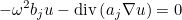
Some parameters can be provided after the description of the incident field, they are starting with a keyword and values:
- Theta Theta : the incident angle θ, by default the value is the value given in the keyword IncidentAngle.
- Phi Phi : the incident angle φ (3-D only), by default the value is the value given in the keyword IncidentAngle.
- Origin x0 y0 z0 : the origin of the plane, by default the value is the value given in the keyword OriginePhase. In 2-D, only two values x0 and y0 must be provided.
- Pulsation omega : the wave number, by default the value is the value given in the keyword Frequency.
- Waist w : the waist of the gaussian, by default the value is equal to 0. As a result, this keyword is needed for gaussian beams (it is not used for other incident fields).
Example :
# angles theta and phi
IncidentAngle = 60.0 40.0

# Plane wave incident field
TypeSource = SRC_DIFFRACTED_FIELD PLANE_WAVE

# origin of the incident field
OriginePhase = 0.0 2.0 0.0

# polarization of the incident field
Polarization = 0.0 1.0 0.0

# incident field with Hankel function
TypeSource = SRC_DIFFRACTED_FIELD HANKEL_WAVE Origin -5.0 0.0 0.0

# incident field with a gaussian beam
TypeSource = SRC_TOTAL_FIELD GAUSSIAN_BEAM Waist 6.4

# Layered incident wave
# LAYERED_PLANE_WAVE nb_layers d0 b0 a0 d1 b1 a1 ... dN
# here two layers at with d = [-0.5, 0.2, 2.5]
TypeSource = SRC_TOTAL_FIELD LAYERED_PLANE_WAVE 2 -0.5  2.0 0.8  0.2 3.0 1.2  2.5
If you choose SRC_TOTAL_FIELD, SRC_DIFFRACTED_FIELD or SRC_USER, only a line TypeSource is necessary to describe the source. For other sources (ie SRC_VOLUME, SRC_SURFACE, SRC_DIRAC and SRC_MODE) , several lines TypeSource can describe the same source. We consider that terms are added
.For SRC_VOLUME, the function f can be chosen among the following list:
- GAUSSIAN x0 y0 (z0) r1 r2 : a gaussian centered at
point (x0, y0, z0) (z0 is not present in 2-D) and with a
distribution radius equal to r1. The gaussian is equal to:
where r is the distance to the center. The parameter alpha is set such that
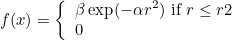 r2 is a cut-off radius. If not provided, it will be set to r1. The parameter beta is given as
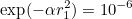

- UNIFORM : an uniform source (f=1). The polarization can be set by writing Polarization followed by values. The source f is constant only on the specified reference, such that you can specify a piecewise constant source if the mesh contains different physical references.
- VARIABLE_BINARY : a variable source. The source is provided directly
on quadrature points of the mesh with a binary file. Quadrature points must be written
by specifying WriteQuadraturePoints=YES. Then, you can
write the source in a binary as follows (in Python, by including visuND package):
# first you read the points contained in file quadrature_points.dat PT = loadtxt('../quadrature_points.dat') x = PT[:, 0] y = PT[:, 1] # then you evaluate your source on these points f = exp(-5.0*(x*x + y*y)) # and write the source in a binary file write_full("../binary_source.dat", f) # if the source has different components, they are written in the same file g = zeros(nb_components*len(x)) f1 = sin(x)*sin(y) f2 = cos(x)*cos(y) ... g[0:len(x)] = f1 g[len(x):2*len(x)] = f2 ... write_full("../binary_source.dat", g) - GRADIENT_BINARY : a variable source to be integrated against gradient of basis functions
(or curl for Maxwell's equations), i.e:
This source has to be evaluated on quadrature points of the mesh in binary (as explained for the previous item VARIABLE_BINARY.

For SRC_SURFACE, the function f can be chosen among the following list:
- GAUSSIAN x0 y0 (z0) r1 r2 : a gaussian centered at point (x0, y0, z0) (z0 is not present in 2-D) and with a distribution radius equal to r1. The gaussian is the same as described above.
- UNIFORM : an uniform source (f=1). The polarization can be set by writing Polarization followed by values.
- INCIDENT_WAVE : the function f is an incident wave, the parameters are the same as those used to described an incident field (see above).
- VARIABLE file_points file_value : the function f is
variable and provided through a list of points and a list of
values. The points are written in a text file while values are
written in binary. Below, we list Python commands to write these two
files (by including visuND package) :
# exemple of a source on boundary y = -2
PT = zeros([N, 2])
PT[:, 0] = linspace(-2.0, 2.0, N)
PT[:, 1] = -2.0*ones(N)
savetxt("Points.txt", PT)

A = zeros([N, 1]) + 1j*zeros([N, 1])
A[:,0] = exp(1j*PT[:,0])
write_full("Values.dat", A)
the matrix A contains values. Each column corresponds to a different component of f. For scalar equations (such as Helmholtz equation), there is only one component to provide.
Example :
# Volume source : GAUSSIAN x0 y0 radius (in 2-D)
TypeSource = SRC_VOLUME GAUSSIAN 0 0 1.0

# Volume source : f = 1 on reference 1 and 0 otherwise
TypeSource = SRC_VOLUME 1 UNIFORM Polarization 1.0

# Volume source : f given directly on quadrature points
# syntax SRC_VOLUME ref VARIABLE_BINARY values.dat
# non null only on reference 2 here
TypeSource = SRC_VOLUME 1 VARIABLE_BINARY binary_source.dat

# case where we compute integral against gradient of basis functions
TypeSource = SRC_VOLUME 1 GRADIENT_BINARY binary_source.dat

# Surface source on reference 2 :
# Polarization can be used to set the amplitude for scalar equations
# TypeSource = SRC_SURFACE 2 GAUSSIAN x0 y0 r1 r2 Polarization p0 ... pN
TypeSource = SRC_SURFACE 2 GAUSSIAN -2.0 0.4  1.0 1.5 Polarization 1.0

# Other surface source on reference 3
TypeSource = SRC_SURFACE 3 UNIFORM Polarization 2.0

# other source for reference 4
TypeSource = SRC_SURFACE 4 INCIDENT_WAVE PLANE_WAVE Theta 60.0 Polarization 0.4

# variable source for reference 5
TypeSource = SRC_SURFACE 5 VARIABLE Points.txt Values.dat

# the right hand side computed is obtained by summing all contributions
Location :
Source/DefineSourceElliptic.cxx
ThresholdRhs
Syntax :
ThresholdRhs = epsilon
The threshold for right hand sides is used to avoid computing the solution of linear systems when the right hand side is considered as negligible. For such linear systems, the solution will be set to 0. The default value is the machine precision (1e-16 for double precision).
Example :
ThresholdRhs = 1e-100
Location :
Source/DefineSourceElliptic.cxx
InitialCondition
Syntax :
InitialCondition = USER param1 param2 ... paramn
No default initial condition is implemented in Montjoie, except null initial conditions. However, you can enter the initial condition by modifying the file UserSource.cxx, but you will need to recompile Montjoie for each modification of the initial condition. Nevertheless, you can provide parameters after USER, so that you can reuse those parameters in the file UserSource.cxx.
Example :
# after USER you can give any number of parameters
InitialCondition = USER 2.0
Location :
Instationary/VarInstationary.cxx
TemporalSource
Syntax :
TemporalSource = type_source parameters
Most often in Montjoie, we consider source with separated variables, i.e. obtained by multiplying a function F(t) depending on time with a function g(x) depending on space. For example, for the wave equation, we consider the first-order system:
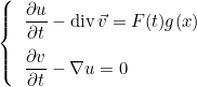
The space source g(x) is defined by the keyword TypeSource while the time source F(t) is defined by the keyword TemporalSource. F(t) is usually the primitive of a function f(t), since the equivalent second-order formulation of the wave equation reads:
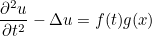
As a result, the obtained solution will be the same with schemes adapted to the first-order system or with schemes adapted to the second-order equation. Some predefined functions are available to specify F(t), they use the frequency defined by the keyword Frequency. You can also provide your own time source, either with an ASCII file containing a list of values, or by modifying the file UserSource.cxx. There is no default value, null source will be computed if you don't insert this field. The following time sources are available (parameters are written in italic) :
- RICKER : a Ricker (i.e. second-derivative of a
gaussian) :
The frequency f0 is the central frequency of the Ricker
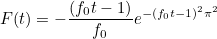
- MODIFIED_RICKER t0 : a Ricker with a center time
t0
The center time t0 is provided as the first parameter.
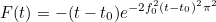
- GAUSSIAN w0 : a gaussian with a center plateau of
width w0 (initial time t0 is equal to 0)
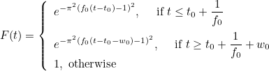
- HARMONIC T0 : a sine function with smooth cut-off,
T0 is the final time of the source.
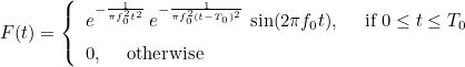
- SINUS_GAUSSIAN alpha : a gaussian (with parameter
alpha) modulated
by a sine function:
The time t0 is initialized such that
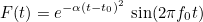

- FILE file_name t0 tf : the function F(t) is
given with values contained in a file. The first parameter is the
file name, the two other parameters are the initial time and final
time. The values of the source are assumed to be known at
equidistributed times :
where
 N is the number of values stored in the file. The file contains an unique column with only values (in text file) :
 F(t) is then computed for any time t by a cubic interpolation.
- USER parameters : F(t) is given by the user in the file UserSource.cxx (method Evaluate of the class TimeUserSource). The parameters can be used in the constructor of the class TimeUserSource.
For the wave equation (targets acous2D and acous3D), an incident plane wave can be specified (TypeSource = SRC_DIFFRACTED_FIELD or SRC_TOTAL_FIELD). In that case, the source is not written in separated variables. The incident plane wave is given as
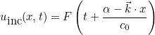
where F is the time source (as specified by the keyword
TemporalSource),
 is the wave vector (given through the frequency and the incident
angles), c0 is the velocity of the media at infinity. The
parameter alpha is equal to:
is the wave vector (given through the frequency and the incident
angles), c0 is the velocity of the media at infinity. The
parameter alpha is equal to:

if AUTO has been selected in TypeSource:
TypeSource = SRC_TOTAL_FIELD AUTO
otherwise it is equal to the parameter given by the user (instead of AUTO). The source is deduced from the definition of the incident wave (for a total field, it implies a source in PML or ABC).
Example :
# a gaussian with a plateau of width=0.2
TemporalSource = GAUSSIAN 0.2

# exp(-alpha (t-t0)^2) * sin (2 pi f t)
TemporalSource = SINUS_GAUSSIAN 0.2

# values given on a file
TemporalSource = FILE source.dat 0 10
Location :
Instationary/VarInstationary.cxx
TimeStep
Syntax :
TimeStep = dt
The time step is provided in this field, otherwise the default value is equal to 0.01. If dt is set to AUTO, the CFL will be computed by evaluating the maximal eigenvalue of M-1 K (where M is the mass matrix and K the stiffness matrix). This operation is expensive, but sometimes it can be interesting to have a good estimate of the CFL. Once the CFL is evaluated, the time step is then chosen close to the CFL limit (0.999 CFL).
Example :
TimeStep = 0.1

# automatic choice of TimeStep by evaluating CFL
TimeStep = AUTO

# you can also choose the time duration and the number of iterations
# the time step will be equal to   Time Duration / Number iterations
# TimeStep = DIVISION Tfinal nb_iterations
TimeStep = DIVISION 10.0  200
Location :
Instationary/VarInstationary.cxx
TimeInterval
Syntax :
TimeInterval = t0 tf
You can specify the final time tf and initial time t0 of the experience. Default values are set to 0.
Example :
TimeInterval = 0 100
Location :
Instationary/VarInstationary.cxx
RandomInitialCondition
Syntax :
RandomInitialCondition = Small
You can specify that the initial condition is set with small random values (usually of 1e-270). It happens that the simulation can be slow at the beginning because of a null initial condition. Indeed, denormal values appear and slow the computation. To overcome this problem, you can start from a non-null initial condition with these small random values. Another possibility is to compile with some options in order to prohibit denormal values:
// in your program, you add these lines
#include <xmmintrin.h>

#define CSR_FLUSH_TO_ZERO         (1 << 15)

// in the main program, you have to add these lines
int main()
{
   unsigned csr = __builtin_ia32_stmxcsr();
   csr |= CSR_FLUSH_TO_ZERO;
   __builtin_ia32_ldmxcsr(csr);

}
Example :
RandomInitialCondition = Small
Location :
Instationary/VarInstationary.cxx
DisplayRate
Syntax :
   DisplayRate = N
   DisplayRate = N YES
The norm of the solution is display each N iterations. You can set N with this field. By default, N depends on the print level chosen. If the second optional parameter is present, the computational time is also displayed.
Example :
# each ten iterations, the norm of the solution is displayed
DisplayRate = 10

# you can also display computational time
DisplayRate = 10 YES
Location :
Instationary/VarInstationary.cxx
LoadReprise
Syntax :
LoadReprise = YES
If asked, the code will try to read the data saved in a previous simulation and resume the simulation from the last iterate saved.
Example :
LoadReprise = YES
Location :
Instationary/VarInstationary.cxx
SaveReprise
Syntax :
SaveReprise = nb_iter
If present, the code will save data needed to resume the simulation later. The data will be saved each nb_iter iterations. By default, the code does not save anything, and the simulation can not be resumed.
Example :
# data is written on the disk each 100 iterations
SaveReprise = 100
Location :
Instationary/VarInstationary.cxx
PathReprise
Syntax :
PathReprise = directory
The user can provide the directory where datas needed to resume a simulation should be written. It can be interesting to specify a local directory in order to have a fast writing.
Example :
# temporary data is written on /scratch
PathReprise = /scratch
Location :
Instationary/VarInstationary.cxx
NormeMaxSolution
Syntax :
NormeMaxSolution = value
The user can provide a maximal norm allowed for the solution. This value is used to determine if the time scheme is stable or not. If the norm of the solution is greather than this value, the simulation is stopped (in order to avoid slow computations with NaNs). By default, the maximal norm allowed is set to 1e30.
Example :
# If you want to specifiy a different maximal norm
NormeMaxSolution = 100.0
Location :
Instationary/VarInstationary.cxx
OrderTimeScheme
Syntax :
OrderTimeScheme = order type_scheme
Here you provide the time scheme and order. Available time schemes are :
| Scheme | Available orders | First-order Formulation | ABC/Damping | Stable |
| LEAP_FROG_TRUE | 2 | Yes | No | CFL |
| LEAP_FROG | 2 and 4 | No | Yes | CFL |
| OPTIMAL_LEAP_FROG | 2 r | No | Yes | CFL |
| LEAP_FROG_PML | 2 and 4 | Yes | Yes | CFL |
| OPTIMAL_LEAP_FROG_PML | 2 r | Yes | No | CFL |
| NYSTROM | 2 r | Yes | No | No |
| RUNGE_KUTTA_NYSTROM | from 2 to 12 | No | No | CFL |
| SYMMETRIC_MULTISTEP | 2 r | No | No | CFL |
| IMPLICIT_SYMMETRIC_MULTISTEP | 2 r | No | No | CFL |
| ADAMS_BASHFORTH | r | Yes | Yes | CFL |
| ADAMS_BASHFORTH_MOULTON | r | Yes | No | No |
| TALEZER | r | Yes | Yes | CFL |
| RUNGE_KUTTA | from 1 to 8 | Yes | Yes | CFL |
| RUNGE_KUTTA_LOW | 4 | Yes | Yes | CFL |
| GAUSS_RUNGE_KUTTA | 2 r | Yes | Yes | Always |
| THETA_SCHEME | 2 | No | Yes | Always |
| SDIRK | From 1 to 5 | Yes | Yes | Always |
| DIRK | 4 | Yes | Yes | Always |
| CRANK_NICOLSON | 2 | Yes | Yes | Always |
| ADAMS_IMPLICIT | r | Yes | Yes | No |
| MILNE_SIMPSON | r | Yes | Yes | No |
| BDF | r | Yes | Yes | No |
| PADE | 2 r | Yes | Yes | Always |
Some schemes can be unavailable for a given equation. The default value is second order leap frog scheme. Some time schemes need additional parameters, time schemes are detailed in this section.
Example :
TimeScheme = 2 LEAP_FROG_PML
TimeScheme = 4 LEAP_FROG
TimeScheme = 4 RUNGE_KUTTA_LOW

# you need to specify teta here
TimeScheme = 2 THETA_SCHEME 0.25
Location :
ParametersRCS
Syntax :
ParametersRCS = YES ref AUTO MONOSTATIC
ParametersRCS = YES ref order BISTATIC
The computation of radar cross section can be done for Helmholtz and time-harmonic Maxwell equations. Monostatic or bistatic radar cross sections are available. The surface where the computation of the integral is performed is defined by the number ref. This number is not a reference number, but a body number, that can include several reference numbers. order is the order of integration used to evaluate integrals. If AUTO is selected, the order will be taken equal to the order of approximation. The default value is NO (no radar cross section is computed).
Example :
# Body is defined with TypeBody
# TypeBody = ref num_body
# here body 1 is formed with references 2 and 3
TypeBody = 2 1
TypeBody = 3 1

# ParameterRCS = YES num_body AUTO type_rcs
ParametersRCS = YES 1 AUTO BISTATIC

# AngleRCS = teta0 teta1 nb_angles
AngleRCS = 0.0 180.0 181

# file where rcs will be stored
FileRCS = RcsDisque.dat
Location :
Harmonic/TransparencyCondition.cxx
AngleRCS
Syntax :
AngleRCS = teta0 teta1 nb_points
Usually radar cross section is computed between two angles teta0 and teta1 and with a given number of angles (nb_points). The angles should be expressed in degrees. The default values are 0, 180 degrees and 181 points (so that the RCS is computed at every degree).
Example :
AngleRCS = 0.0 180.0 361
Location :
Harmonic/TransparencyCondition.cxx
FileRCS
Syntax :
FileRCS = file_name
FileRCS = file_name file_far_field
The radar cross section will be saved in this file. The default value is "rcs.dat" . If a second argument is specified, the far field is also stored (the far field is the complete vector for Maxwell's equations).
Example :
# by default only radar cross section will be stored
FileRCS = Rcs.dat

# you can give a file name for the far field
FileRCS = Rcs.dat FarField.dat
Location :
Harmonic/TransparencyCondition.cxx
TransparencyCondition
Syntax :
TransparencyCondition = YES ref AUTO
TransparencyCondition = YES ref order
TransparencyCondition = YES ref order ref_domain
For Hemholtz and time-harmonic Maxwell equations, it is possible to use a transparent condition (instead of PML or ABC), which is exact but relies on the representation formula to iterate on the solution. This transparent condition is detailed in M. Durufle's thesis (and in a paper of C. Hazard and M. Lenoir). For the representation formula, a direct integration is used, no multipole strategy is exploited. ref is a body number, you can specify an order of integration, AUTO correspond to selecting the order of approximation. ref_domain is an optional parameter that gives the reference of the volume contained between the artificial boundary and the extern boundary.
Example :
# Body is defined with TypeBody
# TypeBody = ref num_body
# here body 1 is formed with references 2 and 3
TypeBody = 2 1
TypeBody = 3 1

# TransparencyCondition = YES num_body order
TransparencyCondition = YES 1 AUTO
Location :
Harmonic/TransparencyCondition.cxx
ParamResolutionTransparency
Syntax :
ParamResolutionTransparency = type_resolution nb_iterations tolerance restart
The use of transparent condition requires an iterative solver. type_resolution informs the type of iterative solver, nb_iterations the maximum number of iterations, tolerance the stopping criterion and restart the restart parameter (for GMRES for example). Be careful to select an iterative solver which works for unsymmetric linear systems. The default solver is GMRES(10) with a maximum of 100 iterations and a stopping criterion equal to 1e-6. The number of iterations is usually small, especially when the distance between the extern boundary and the intern boundary (on which representation formula is computed) is large.
Example :
# ParamResolutionTransparency = algo nb_iter_max  epsilon  restart_parameter
ParamResolutionTransparency = GMRES 100 1e-6 10
Location :
Harmonic/TransparencyCondition.cxx
TypeBody
Syntax :
TypeBody = ref body1 body2 ... bodyn
You can group surfaces of different references into a single body (with a unique number). This body number is then used for the computation of radar cross section or for the transparent condition. By default, no body is created.
Example :
# Body 2 includes surfaces of reference 2 and 3
# Body 1 includes surfaces of reference 1 and 3
TypeBody = 1  1
TypeBody = 2  2
TypeBody = 3  1 2
Location :
ExplicitMatrixFEM
Syntax :
ExplicitMatrixFEM = YES_NO_or_AUTO
If the value is YES, the finite element matrix will be effectively computed even though it is not needed. If the value is NO, and if an iterative solver (for time-harmonic simulations) is selected or for explicit time-stepping (for time-domain simulations), the finite element matrix is not computed. The matrix-vector product is made with a matrix-free implementation. Usually only the jacobian matrices DFi are stored and used for this matrix-vector product. If the value is AUTO, the code will choose if the finite element matrix is stored or not.
Example :
# if you want that the finite element matrix is computed
ExplicitMatrixFEM = YES
Location :
StorageMatrix
Syntax :
StorageMatrix = YES nom_fichier
During the computation, the finite element matrix can be stored in a file, so that you can check that the computation is correctly done. It is better to use a direct solver if you want to store the matrix in a file, because if you choose an iterative solver, this will probably perform a matrix vector product will all canonical vectors (1,0,...0), (0,1,0, ...,0), ..., (0,0, ...,1). And this can be very long if the matrix is large. But this is also a way to check that the matrix-free implementation is correctly implemented for the finite element and equation you consider. If the file name ends with mtx, the matrix will be stored in the MatrixMarket format. The default value is set to NO.
Example :
#if you want to store the matrix in the file mat.dat
StorageMatrix = YES mat.dat

# to write the FEM matrix in MatrixMarket format, use the extension mtx
StorageMatrix = YES mat.mtx
Location :
ThresholdMatrix
Syntax :
ThresholdMatrix = tolerance
If you hope to obtain a sparser matrix, you can set a threshold, and all the entries of the matrix smaller than this threshold won't be added to the matrix during assembly phase.
Example :
ThresholdMatrix = 1e-6
Location :
PrintLevel
Syntax :
PrintLevel = level
This entry can be modified if you want to increase or decrease the level of displayed messages. A value of -1 will display nothing (silent mode). The default value is 0. The maximum value is 10 but displays a lot of informations and writes stuff on the disk. An intermediate value is 6 and is better in a normal use.
Example :
PrintLevel = 2
Location :
WriteQuadraturePoints
Syntax :
WriteQuadraturePoints = YES/NO
WriteQuadraturePoints = YES NO_PML_POINTS
If you specify YES, quadrature points will be written in the file quadrature_points.dat. If the simulation is launched with several processors, the quadrature points of each processor will be written in a separated file : quadrature_points_P0.dat, quadrature_points_P1.dat, etc. The second argument NO_PML_POINTS is optional. If present, quadrature points of elements in PML elements will not be written.
Example :
WriteQuadraturePoints = YES
Location :
Harmonic/VarGeometryProblem.cxx
EnergyConservingAeroacousticModel
Syntax :
EnergyConservingAeroacousticModel = type_model
This entry sets which model is used for aeroacoustics (target aero2D, harmonic_aero2D). The following models are available:
- YES : conservative model (an energy is conserved)
- BogeyBaillyJuve : Bogey-Bailly-Juve model
- Galbrun : simplified Galbrun's equation
- NO : simplified Linearized Euler's equation
Example :
EnergyConservingAeroacousticModel = Galbrun
Location :
Elliptic/AeroAcoustic/AeroAcoustic.cxx
DropUnstableTerms
Syntax :
  DropUnstableTerms = Convective
  DropUnstableTerms = Convective alpha
  DropUnstableTerms = NonUniform
This entry can be used to drop some terms for target galbrun_axi
Example :
DropUnstableTerms = Convective 0.2
Location :
Elliptic/AeroAcoustic/AxiSymGalbrun.cxx
ApplyConvectiveCorrectionSource
Syntax :
ApplyConvectiveCorrectionSource = YES
This entry can be used to apply convective derivative to the volume source:
Example :
ApplyConvectiveCorrectionSource = YES
Location :
Elliptic/AeroAcoustic/AxiSymGalbrun.cxx
ForceFlowNeumann
Syntax :
ForceFlowNeumann = YES/NO
If specified to YES, the Neumann condition will be enforced. Usually, Neumann condition will be weakly satisfied by the steady flow (computed by a Discontinous Galerkin method for example). As a result, Neumann condition is approximately verified, and this can produce numerical instabilites, that are removed by enforcing a strongly Neumann condition. If no entry is provided, this operation is not performed, default value is NO.
Example :
ForceFlowNeumann = YES
Location :
Elliptic/AeroAcoustic/HarmonicGalbrun.cxx
NumberModes
Syntax :
  NumberModes = AUTO tolerance
  NumberModes = AUTO tolerance nb_min_modes
  NumberModes = SINGLE num_mode
  NumberModes = nb_modes
For the finite element solution in an axisymmetric configuration, each Fourier mode is solved separately. The selection of Fourier modes to solve can be automatically performed by specifying tolerance. When the norm of the right hand side is lower than tolerance (in relative value), the computation is stopped. You can also specify a maximum number of modes nb_modes, and all the modes between -nb_modes and nb_modes will contribute to the solution. Default value is automatic selection of number of mondes with tolerance equal to 1e-6.
Example :
# computation will be stopped when the norm of x_m will be smaller than 1e-12 max || x_i ||
NumberModes = AUTO 1e-12

# you can enforce the computation of first modes (in order to compute correctly the maximum)
NumberModes = AUTO 1e-12 8

# you can specify the number of modes to compute
NumberModes = 20

# you can ask the solution for a single mode
NumberModes = SINGLE 1
Location :
ForceDiagonalMass
Syntax :
ForceDiagonalMass = YES
For axisymmetric Helmholtz equation, the mass matrix can be lumped by using Gauss-Radau points. This functionality can be triggered with this keyword.
Example :
# diagonal mass matrix
ForceDiagonalMass = YES
Location :
AddFlowTerm
Syntax :
AddFlowTerm = YES
For Helmholtz equation, a convection term can be added if this keyword is present. If the value is set to YES, Helmholtz equation is given as:

The default value is NO (the flow M is assumed to be zero).
Example :
# first, you need to say that a convection term is present
AddFlowTerm = YES

# then you can specify a flow for the different domains
PhysicalMedia = M 1 ISOTROPE 0.5 0.0
Location :
Elliptic/Helmholtz/VarHelmholtz.cxx
AddSlot
Syntax :
AddSlot = x0 y0 x1 y1 epsilon N
For 2-D Helmholtz equation, if MONTJOIE_WITH_THIN_SLOT_MODEL has been defined in the compiled file (or with faster compilation), you can specify a thin slot in the computational domain. The thin slot extends between points [x0, y0] and [x1,y1], with a thickness epsilon.
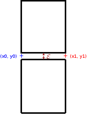
First-order models are used, a Dirichlet-to-Neumann model or a 1-D model (which avoids the problem of resonant frequencies). For more details about the used models, you can read S. Tordeux's thesis. N denotes the number of points to discretized the 1-D solution along the slot (used in the case of 1-D model). There is no default value since no slot is included at the beginning.
Example :
# specify a slot of extremities [0,0] [2,0] and of thickness 0.1
AddSlot = 0 0 2 0 0.1 200
# you can add as many slots as you want with different parameters
AddSlot = -1 -2 1 -2 0.2 100
Related topics :
Location :
Elliptic/Helmholtz/VarHelmholtz.cxx
ModelSlot
Syntax :
ModelSlot = DTN/MESH_1D
For 2-D Helmholtz equation, if MONTJOIE_WITH_THIN_SLOT_MODEL has been defined in the compiled file, you can specify a thin slot in the computational domain. First-order models are used, a Dirichlet-to-Neumann model or a 1-D model (which avoids the problem of resonant frequencies). For more details about the used models, you can read S. Tordeux's thesis. DTN corresponds to the Dirichlet-to-Neumann model while MESH_1D corresponds to the 1-D model. Default value is MESH_1D.
Example :
ModelSlot = DTN
Related topics :
Location :
Elliptic/Helmholtz/VarHelmholtz.cxx
CalculEnveloppe
Syntax :
CalculEnveloppe = YES
For axisymmetric Helmholtz equation (target helm_axi), you can ask to compute the enveloppe, i.e. the field v such that :
It can be interesting if the wave propagates mainly in z-direction
Example :
CalculEnveloppe = YES
Location :
Elliptic/Helmholtz/AxiSymHelmholtz.cxx
FormulationAxisymmetric
Syntax :
FormulationAxisymmetric = R3
For axisymmetric Helmholtz equation, the usual variational formulation (without flow term) is equal to :

There is no singularity because an homogeneous Dirichlet condition is set on the axis for m different from 0. If the formulation R3 is selected, we replace basis functions as:

It implies the following variational formulation

This formulation is denoted R3 because of the presence of r3 weight for the mass matrix. With this variational formulation, Dirichlet condition is no longer enforced, and we have only polynomials in r.
Example :
# if you want to use the r^3 formulation
FormulationAxisymmetric = R3
Location :
Elliptic/Helmholtz/AxiSymHelmholtz.cxx
TimeReversal
Syntax :
TimeReversal = DIRECT t0 tf dt fichier_maillage fichier_du_dn ref
TimeReversal = INVERSE t0 tf dt fichier_maillage fichier_du_dn ref
This entry gives the possibility to simulate time reversal experiences. It is currently only available for 2-D acoustic equation, but the extension would be straightforward for other equations. If you specify DIRECT, the values of du/dn are computed on a boundary of reference ref and stored in the file fichier_du_dn each dt. Then, you can use these datas (modify them if you want), to simulate a time reversal (INVERSE). The same parameters should must be kept (t0, tf, ...). fichier_maillage contains a mesh of the boundary. The reference can change, since the mesh can be different in direct and inverse experiences. There is no default value, time reversal is optional.
Example :
TimeReversal = DIRECT 10.0 20.0 0.1 boundary.mesh dudn.dat 2
TimeReversal = INVERSE 10.0 20.0 0.1 boundary.mesh dudn.dat 4
Location :
Hyperbolic/Acoustic/TimeReversal.cxx
FileCoefficientsQ
Syntax :
FileCoefficientsQ = file_name
This entry allows the user to compute coefficients Qi:
for each element i. These coefficients are written in an output file. By default, such coefficients are not computed.
Example :
# if you want to compute q_i and store them:
FileCoefficientsQ = file_Qi.dat
Location :
Elliptic/Maxwell/3D/HarmonicMaxwell3D.cxx
ModifiedFormulation
Syntax :
ModifiedFormulation = YES
This entry enables the user to use a modified formulation for axisymmetric Maxwell's equations. Usually, this formulation is more accurate. By default, this formulation is not selected.
Example :
ModifiedFormulation = YES
Location :
Elliptic/Maxwell/Axi/AxiSymHcurlMaxwell.cxx
OutputHy
Syntax :
OutputHy = ref0 .. refN PARAM file_name n
By inserting this line, the user asks to write Hy on a set of referenced curves. n is the number of subdivisions for each interval.
Example :
# on edges of reference 2 and 3, Hy is computed with 10 subdivisions for each edge
OutputHy = 2 3 PARAM Hy.dat 10
Location :
Elliptic/Maxwell/Axi/MaxwellAxiSymHarmonic.cxx
DisplayStress
Syntax :
DisplayStress = NO
For elastodynamics equations, it may be interesting to display the stress σ :

when the gradient is required. If NO is selected, the gradient of u is displayed, otherwise the stress is displayed. The default value is YES, if this line is not present the stress is displayed.
Example :
# if you want to know the gradient of u, and not the stress :
DisplayStress = NO
Location :
Elliptic/Elastic/VarElastic.cxx
ThicknessPlate
Syntax :
ThicknessPlate = delta
ThicknessPlate = VARIABLE ref param_media
The thickness of the plate is specified, otherwise the default value is 0.1. It is only used for Reissner-Mindlin equations. For a variable thickness the parameters are detailed in the description of MateriauDielec.
Example :
ThicknessPlate = 0.1

# for a variable thickness
ThicknessPlate = VARIABLE 1 SAME_MESH test_plaque.mesh 0.0 1.0 delta.don 8 0.02
Location :
Hyperbolic/Elastic/ReissnerMindlin.cxx
SismoPlane
Syntax :
# for 2-D and axisymmetric targets
SismoPlane = AUTO nx ny
SismoPlane = xmin xmax ymin ymax nx ny

# 3-D targets
SismoPlane = x0 y0 z0 xA yA zA xB yB zB nx ny
Solution can be computed on a plane, on the rectangle [xmin, xmax] x [ymin, ymax] in 2-D, and on the parallelogram defined by the origin (x0, y0, z0) and the two extremities (xA, yA, zA), (xB, yB, zB) in 3-D. nx and ny are the number of points along direction x and direction y. By default, no output is done on planes. In 2-D, AUTO means that the code will use the bounding box of the physical domain (PML layers are excluded).
Example :
# for regular grids in 2-D
SismoPlane = AUTO 101 101
SismoPlane = -5 5 -5 5  101 101

# for 3-D plane {0} x [-1, 1] x [0 2]
SismoPlane = 0 -1  0   0 1 0   0 -1  2  101 101
Location :
SismoPlaneAxi
Syntax :
# axisymmetric targets
SismoPlaneAxi = x0 y0 z0 xA yA zA xB yB zB nx ny
Solution can be computed on a 3-D parallelogram defined by the origin (x0, y0, z0) and the two extremities (xA, yA, zA), (xB, yB, zB) in 3-D. nx and ny are the number of points along direction x and direction y.
Example :
# for output on a 3-D plane {0} x [-1, 1] x [0 2] for axisymmetric case
SismoPlaneAxi = 0 -1  0   0 1 0   0 -1  2  101 101
Location :
SismoGrille
Syntax :
# output on three planes intersecting at point (x0, y0, z0)
SismoGrille = x0 y0 z0 AUTO nx ny nz
SismoGrille = x0 y0 z0 xmin xmax ymin ymax zmin zmax nx ny nz
3-D solutions can be computed on three planes : {x0} x [ymin, ymax] x [zmin,zmax], and [xmin, xmax] x {y0} x [zmin, xmax] and [xmin, xmax] x [ymin,ymax] x {z0}. The number of points on each direction are nx, ny and nz. If AUTO is specified, the code uses the bounding box of the physical domain (PML layers are excluded).
Example :
# AUTO : bounding box is the bounding box of the mesh
SismoGrille = 0 0 0 AUTO 101 101 101
Location :
SismoLine
Syntax :
# output on the line joining A to B
SismoLine = xA xB yA yB nb_points

# For 3-D
SismoLine = xA xB yA yB zA zB nb_points
Output on lines of extremities (xA, yA, zA) and (xB, yB, zB) can be performed, nb_points is the number of points on the line.
Example :
# Line x = 2, y in [0, 10]
SismoLine = 2 2 0 10 201
Location :
SismoLineAxi
Syntax :
# output on a 3-D line
For 3-D
SismoLine = xA xB yA yB zA zB nb_points
Output on 3-D lines of extremities (xA, yA, zA) and (xB, yB, zB) can be performed, nb_points is the number of points on the line. This field is meaningful only for axisymmetric targets.
Example :
# Line x = 2, y in [0, 10], z in [-4, 4]
SismoLineAxi = 2 2 0 10 -4.0 4.0 201
Location :
SismoCircle
Syntax :
# 2-D circles
SismoCircle = x0 y0 radius nb_points

# 3-D circle
SismoCircle = x0 y0 z0 nx ny nz ra rb nb_points
In 2-D, you specify the center and radius of the circle. In 3-D, you specify the center (x0, y0, z0) of the circle, the normale (nx, ny, nz) of the plane containing the circle, and ra, rb the two radii (for an ellipse). nb_points is the number of points in the circle.
Example :
# output on a circle of center (0, 0) and radius 3 with 201 points
SismoCircle = 0 0  3.0  201
Location :
SismoCircleAxi
Syntax :
# 3-D circle
SismoCircleAxi = x0 y0 z0 nx ny nz ra rb nb_points
The solution can be computed on points on a 3-D ellipse. This field is meaningful only for axisymmetric targets. nx, ny, nz denotes the normale to the plane where the circle lies. ra and rb are two radii.
Example :
SismoCircleAxi = 0 0 0 1 0 0 3.0 5.0 201
Location :
SismoPoint
Syntax :
# 2-D point
SismoPoint = x0 y0

# 3-D point
SismoPoint = x0 y0 z0
You can compute the solution on a single point ... This is actually useful for time-domain simulations in order to obtain a seismogramm. In this case, the output is written in the SAME file and in ASCII format so that you can directly read the file in Matlab by using command load (or in gnuplot). If you insert several SismoPoint, the solution will be computed on all the points given, as explained in FileOutputPoint.
Example :
SismoPoint = 2 0
Location :
SismoPointAxi
Syntax :
# 3-D point
SismoPointAxi = x0 y0 z0
You can compute the solution on a single 3-D point ... This is actually useful for time-domain simulations in order to obtain a seismogramm. In this case, the output is written in the SAME file and in ASCII format so that you can directly read the file in Matlab by using command load (or in gnuplot). If you insert several SismoPoint, the solution will be computed on all the points given, as explained in FileOutputPoint. This field is meaningful only for axisymmetric targets.
Example :
SismoPointAxi = 2 0 0.8
Location :
SismoPointsFile
Syntax :
SismoPointsFile = nom_fichier
The solution can be computed on points defined by the user. In that case, you have to provide a file in ASCII format, like that :
x0 y0 z0
x1 y1 z1
...
In 2-D, of course you have only two coordinates to give.
Example :
SismoPointsFile = points.dat
Location :
SismoPointsFileAxi
Syntax :
SismoPointsFileAxi = file_name
The solution can be computed on 3-D points defined by the user. In that case, you have to provide a file in ASCII format, like that :
x0 y0 z0
x1 y1 z1
...
This field is meaningful for axisymmetric targets only.
Example :
SismoPointsFileAxi = points.dat
Location :
SismoGrille3D
Syntax :
# output on 3-D regular grid [xmin, xmax] x [ymin, ymax] x [zmin, zmax]
SismoGrille3D = AUTO nx ny nz
SismoGrille3D = xmin xmax ymin ymax zmin zmax nx ny nz
3-D solutions can be computed on the 3-D grid [xmin, xmax] x [ymin,ymax] x [zmin, zmax]. The number of points on each direction are nx, ny and nz. In our opinion, you have to be careful, because such output files are very expensive in memory. If you ask 200 points in each direction with complex double precision, a single file will take 122 Mo ... That's why it is often better to compute solution only on three planes by using the keyword SismoGrille. If AUTO is specified, the codes uses the bounding box of the physical domain (PML layers are excluded).
Example :
SismoGrille3D = AUTO 101 101 101
Location :
OutputFormat
Syntax :
OutputFormat = BINARY/ASCII FLOAT/DOUBLE
Actually only binary files are usable since in Matlab, there are no script files to read ascii files produced by Montjoie . Furthermore, seismogramms on points and radar cross sections are written in ASCII and directly readable with Matlab by using command load. The binary files can be written in simple precision (FLOAT) or double precision (DOUBLE), both formats are correctly interpreted in Matlab (by script loadND). You can also ask outputs in vtk format (readable by Paraview), BINARY has to be replaced by VTK and ASCII by ASCII_VTK. The default format is BINARY DOUBLE.
Example :
# outputs in "Matlab" format and medit for mesh outputs
OutputFormat = BINARY DOUBLE
OutputFormat = BINARY FLOAT

# For outputs in vtk format only :
OutputFormat = VTK DOUBLE
Location :
DirectoryOutput
Syntax :
DirectoryOutput = AUTO
DirectoryOutput = path
The user can specify the directory where output files will be written. If equal to AUTO, the output files will be written in [STIFFOUT]/num where num is a number that will be incremented for each next simulation. The default value is ./ (output files are written in the current directory).
Example :
# Directory where output files are written
DirectoryOutput = /home/user/Results/
Location :
ElectricOrMagnetic
Syntax :
ElectricOrMagnetic = component
This field is useful to select the component of the solution (and the gradient/curl) you want to know. If you wish to see all the components and gradients, you will put -1, whereas a positive integer will select a single component. If you want only components of the solution (and not gradients), put -2. The default component is 0 (so only the first component of solution). If you want to compute all the components of the solution, gradients and also hessians, you have to put -5. The hessians are computed through an interpolation on nodal points.
Example :
# all the components of the solution
ElectricOrMagnetic = -1

# all the components of the solution but not the gradients
ElectricOrMagnetic = -2

# only Ez for example
ElectricOrMagnetic = 2

# if you want to have all components, gradients and hessians
ElectricOrMagnetic = -5
Location :
FineMeshLobatto
Syntax :
FineMeshLobatto = YES
You can require to compute the values of the solution on the nodal values of the mesh. Instead of subdividing the mesh in regular subdivisions, you subdivide it on Gauss-Lobatto points, so that the vertices of the fine are coincident with the nodal points. The default value is NO.
Example :
FineMeshLobatto = YES
Location :
WriteSolutionQuadrature
Syntax :
WriteSolutionQuadrature = YES file_name_solution file_name_weights
You can require to compute the values of the solution on the quadrature points of the mesh. The second parameter is the file name where the solution will be written. The third parameter is the file name where the quadrature weights will be written. They can be read in Python by typing
  u = load1D('sol.dat');
  w = load1D_real('poids.dat');
Example :
WriteSolutionQuadrature = YES sol.dat poids.dat
Location :
MovePointsSurface
Syntax :
MovePointsSurface = YES component coef
You can require that outputs on surface meshes are produced with translated points. The second argument is the component number used to translate the point. Z-coordinate of the solution is modified:
where m is the component number. In 2-D computation, a 3-D mesh is generated with a z-coordinate.
Example :
MovePointsSurface = YES 1 0.2
Location :
NonLinearSolver
Syntax :
NonLinearSolver = type_solver threshold nb_max_iteration
With this keyword, you can specify the non-linear solver used to invert transformation Fi. This transformation transforms any reference element into the real element. As a result, it is necessary to invert this transformation when points of output grids are localized in the mesh. The default solver is Newton solver, usually it works pretty well.
Example :
# if you want to specify a different threshold or different maximum number of iterations
NonLinearSolver = NEWTON 1e-14 20

# other solvers are LVM (=Levenberg-Marquardt) and MINPACK
NonLinearSolver = LVM 1e-15 10
NonLinearSolver = MINPACK 1e-15 50
Location :
FiniteElement/PointsReference.cxx
SismoMeshVolumetric
Syntax :
SismoMeshVolumetric = AUTO
SismoMeshVolumetric = nb_subdiv
You can require to compute the values of the solution on a subdivided mesh (with regular subdivisions). The number of subdivisions can be explicitely provided or equal to the order of approximation (AUTO). There is no default value. If FineMeshLobatto is enabled, the subdivisions are based on Gauss-Lobatto points instead of equidistributed points.
Example :
# Output on subdivided mesh with nb_subdiv = 3 for each edge
SismoMeshVolumetric = 3
Location :
SismoMeshSurfacic
Syntax :
SismoMeshSurfacic = AUTO BODY ref1 ref2 ... refn
SismoMeshSurfacic = AUTO CONDITION ref1 ref2 ... refn
SismoMeshSurfacic = AUTO REFERENCE ref1 ref2 ... refn
SismoMeshSurfacic = AUTO REFERENCE ALL
You can require to compute the values of the solution on the surfaces of the mesh (therefore in 3-D only). As for SismoMeshVolumetric, the solution is computed on a regular subdivision of the surfacic mesh. The number of subdivisions can be explicitely provided or equal to the order of approximation (AUTO). You can select all the surfaces of the mesh (REFERENCE ALL), or provide the references of the surface. There is no default value.
Example :
# surfacic mesh of all the surfaces
SismoMeshSurfacic = 3 REFERENCE ALL

# surfacic mesh of surface 1 and 5
SismoMeshSurfacic = AUTO REFERENCE 1 5

# you can ask output on bodies (defined with TypeBody)
SismoMeshSurfacic = AUTO BODY 2

# or on same boundary conditions (but you need to know numbers affected to each boundary condition)
SismoMeshSurfacic = AUTO CONDITION 1
Location :
SismoOutsidePoints
Syntax :
SismoOutsidePoints = file_points file_diffrac file_total dt
SismoOutsidePoints = CIRCLE x0 y0 z0 radius nb_points file_diffrac file_total dt
SismoOutsidePoints = CIRCLE_STEREO x0 y0 z0 radius nb_points dist file_diffrac file_total dt
SismoOutsidePoints = LINE x0 y0 z0 x1 y1 z1 nb_points file_diffrac file_total dt
SismoOutsidePoints = PLANE x0 y0 z0 x1 y1 z1 x2 y2 z2 Nx Ny file_diffrac file_total dt
SismoOutsidePoints = POINT x0 y0 z0 file_diffrac file_total dt
You can require to compute the values of the solution on points located outside the computational mesh (through an integral representation). This functionality is available only for wave equation and Helmholtz equation. You can provide a file containing a list of points or specify points computed on a circle, line or plane. CIRCLE_STEREO corresponds to pairs of points on a circle, the distance between the two points of a pair is given by the user. The last parameter is the time step dt (values are computed each dt), this parameter is not needed for time-harmonic simulations (e.g. Helmholtz equation). The output files are readable in Python/Matlab with the function ReadFarField in time-domain simulation and with loadND for time-harmonic simulation. Of course, in 2-D simulations, the z-coordinate should be omitted in the list of parameters. The surface where the integrals are computed (throught integral representation) is described in ParametersRCS. It is assumed that the media is homogeneous outside this surface (and no source is present). The values of the media at infinity are initialized if you have provided a line with ReferenceInfinity. When a scattered field is computed (diffracted field or total field), only the diffracted field will be computed.
Example :
# To set rho0 and mu0
# you give the reference of the homogeneous media (infinity)
ReferenceInfinity = 1

# the solution is computed through an integral over surface specified with TypeBody/ParametersRCS
TypeBody = 1 1
ParametersRCS = YES 1 AUTO

# you can write all the desired points in a file Points3D.txt
# SismoOutsidePoints = file_points file_diffrac file_total dt
SismoOutsidePoints = Points3D.txt diffracExt.dat totalExt.dat 0.02

# output on points located regularly on a circle
# SismoOutsidePoints = CIRCLE x0 y0 z0 radius nb_points file_diffrac file_total dt
SismoOutsidePoints = CIRCLE 0.0 0.0 0.0   4.0 101 diffracExt.dat totalExt.dat 0.02

# output on pairs of points located regularly on a circle
# SismoOutsidePoints = CIRCLE_STEREO x0 y0 z0 radius nb_points dist file_diffrac file_total dt
SismoOutsidePoints = CIRCLE_STEREO 0.0 0.0 0.0   4.0 101 0.02 diffracExt.dat totalExt.dat 0.02

# output on a single point
# SismoOutsidePoints = POINT x0 y0 z0 file_diffrac file_total dt
SismoOutsidePoints = POINT 0.0 0.0 0.0 diffracExt.dat totalExt.dat 0.02

# output on a 2-D line for a 2-D simulation (you omit the z-coordinates)
# time-harmonic simulation : dt is not needed
# you specify the two extremities of the line (x0, y0) and (x1, y1)
# SismoOutsidePoints = LINE x0 y0 x1 y1 N diffracFile totalFile
SismoOutsidePoints = LINE -3.0 -3.0   3.0 -3.0  501 diffracExt.dat totalExt.dat

# output on a 2-D plane (2-D simulation)
# (x0, y0) is the base of the parallelogramm
# (x1, y1) and (x2, y2) the two points adjacent to (x0, y0)
# Nx and Ny the number of points on each side of the parallelogramm
# SismoOutsidePoints = PLANE x0 y0  x1 y1  x2 y2  Nx Ny diffracFile totalFile
SismoOutsidePoints = PLANE -3.0 -3.0   3.0 -3.0   -3.0 3.0  201 201 diffracExt.dat totalExt.dat
Location :
FileOutputGrille, FileOutputGrille3D, FileOutputPlane, FileOutputLine, etc
Syntax :
FileOutputPlane = nom_fichier_diffrac nom_fichier_total
In this field, you specify the files where the diffracted field and total will be written. All the outputs on planes will be stored in the same file, all the outputs on lines will be in another same file, etc. The exceptions are FileOutputMeshVolumetric, FileOutputMeshSurfacic, which are required AFTER each SismoOutputMeshVolumetric (or SismoOutputMeshSurfacic). In this case, different files are used for the creation of volumetric or surfacic meshes. There is no default value, you need to specify file names.
Example :
# For Matlab files, extension .dat
FileOutputPlane = diffracTest.dat totalTest.dat

# For Medit files, extension .bb
FileOutputMeshVolumetric = diffracTest.bb totalTest.bb
Location :
FileOutputPoint
Syntax :
FileOutputPoint = nom_fichier_diffrac nom_fichier_total
In this field, you specify the files where the diffracted field and total will be written. In the case where there is no diffracted/total field distincition (a simple gaussian source for example), the output is always written in the total field, that is to say the second parameter. For time-domain computations, seismogramms are stored in this file. So the file name is not evolving (0001.dat, 0002.dat) and all the values are stored in the same file, contrary to all other outputs (FileOutputPlane, FileOutputGrille, etc). This seismogramm is usually in ascii format, and can be read by using load function in Matlab (loadtxt in Python). It will look like
t0  u(x0, t0) u(x1, t0) u(x2, t0) ... u(xn, t0)
t1  u(x0, t1) u(x1, t1) u(x2, t1) ... u(xn, t1)
...
tn  u(x0, tn) u(x1, tn) u(x2, tn) ... u(xn, tn)
If ElectricOrMagnetic has been set to a positive value, u(x0, t0) will be equal to the asked component of the solution on the point x0, u(x1, t0) on the point x1, etc. The points x0, x1, ..., xn are given by inserting as many lines "SismoPoint = xi yi" as you want. The order will be the same as the order specified in the data file. If ElectricOrMagnetic has been set to -1, the columns will be the following :
t0  u(x0, t0) u(x1, t0) u(x2, t0) ... u(xn, t0) du(x0, t0) du(x1, t0) du(x2, t0) ... du(xn, t0)
t1  u(x0, t1) u(x1, t1) u(x2, t1) ... u(xn, t1) du(x0, t1) du(x1, t1) du(x2, t1) ... du(xn, t1)
...
tn  u(x0, tn) u(x1, tn) u(x2, tn) ... u(xn, tn) du(x0, tn) du(x1, tn) du(x2, tn) ... du(xn, tn)
where du(x0, t0) will be the gradient of u at point x0. u may have several components and each component is written in a separate column, and du have more components, each component being written in a separate column. If ElectricOrMagnetic has been set to -2, only u is written with all its components.
Example :
# for time-domain computations, first name is not used
FileOutputPoint = diffrac.dat Sismo.dat
Location :
ParametersOutputGrille, ParametersOutputGrille3D, ParametersOutputPlane, ParametersOutputLine, etc
Syntax :
ParametersOutputPlane = t0 tf dt
This field is devoted to transient equations for which snapshots are written at time t in [t0, tf] at every dt. The exceptions are ParametersOutputMeshVolumetric, ParametersOutputMeshSurfacic, which are required AFTER each SismoOutputMeshVolumetric (or SismoOutputMeshSurfacic). In this case, different time intervals can be specified for each output. The default values are set to 0.
Example :
# output for t in [0, 10] for each dt = 0.1
ParametersOutputPlane  = 0.0  10.0  0.1

# for seismograms, you ask a binary output :
ParametersOutputPoint = 0.0 10.0 0.01 BINARY
Location :
DataFileExperiment
Syntax :
DataFileExperiment = input_file ref0 ref1 ... ref_n
This field is devoted for RTM and inverse problems. For these problems, experimental data is needed. This data is generated synthetically by running the case described in the file input_file. The references ref0, ref1 ... ref_n are the references where the solution is measured (on quadrature points).
Example :
# synthetical data is generated by "running" the input file INI/experiment.ini
# and measuring the solution on references 1, 2 and 3
DataFileExperiment = INI/experiment.ini 1 2 3
Location :
DataFileSimulation
Syntax :
DataFileSimulation = input_file ref0 ref1 ... ref_n
This field is devoted for RTM and inverse problems. For these problems, the simulated data and back-propagated data are generated by starting from the case detailed in the file input_file. The references ref0, ref1 ... ref_n are the references where the solution is measured and back-propagated (on quadrature points).
Example :
# simulated and back-propagated data are generated with INI/simu.ini
DataFileSimulation = INI/simu.ini 1 2 3
Location :
TypeSourceLine
Syntax :
TypeSourceLine = nb_source REF ref Gaussian xA yA  xB yB radius rmax
TypeSourceLine = nb_source REF ref PlaneWave tetaA tetaB
TypeSourceLine = nb_source IncidentWave tetaA tetaB
This field is devoted for RTM and inverse problems. It defines a sequence of sources (usually along a line). nb_source is the number of sources, ref is the reference (for surface sources) associated with the surface. Gaussian specifies surface Gaussian sources, and the center of gaussians describes the line between two points. PlaneWave speficies a surface plane wave source, the incident angle will describe the given interval [tetaA, tetaB]. Finally IncidentWave is used to specify a total field source with different incident angles.
Example :
# example with 2-D simulation and gaussian
# 20 sources between points (-2, 2) and (4, 2)
# radius of the Gaussian : 0.1
# 0.2 is a cut-off radius (the gaussian is truncated for r ≥ 0.2)
TypeSourceLine = 20 REF 1 Gaussian -2.0 2.0  4.0 2.0   0.1 0.2

# instead of a Gaussian, you can put a plane wave exp(i k x)
# where k = omega/c (cos teta, sin teta)
# 20 sources with teta between 30 and 120 degrees :
TypeSourceLine = 20 REF 1 PlaneWave 30.0 120.0

# incident field (the total field will be computed)
# the incident wave will be a plane wave
TypeSourceLine = 20 IncidentWave 30.0 120.0
Location :
TypeSourceCircle
Syntax :
TypeSourceCircle = nb_source REF ref Gaussian xA yA radiusA tetaA tetaB radius rmax
This field is devoted for RTM and inverse problems. It defines a sequence of sources (usually along a circle). nb_source is the number of sources, ref is the reference (for surface sources) associated with the surface. Gaussian specifies surface Gaussian sources, the center of the gaussians describes a circle of center (xA, yA) and radius radiusA, with the two angles tetaA and tetaB. radius and rmax are the radii of the Gaussian.
Example :
# example with 2-D simulation and gaussian
# 20 sources in a circle of center (0,0) and radius 2
# half-circle => angles between 0 and 180
# radius of the Gaussian : 0.1
# 0.2 is a cut-off radius (the gaussian is truncated for r ≥ 0.2)
TypeSourceCircle = 20 REF 1 Gaussian 0.0 0.0 2.0  0.0  180.0   0.1 0.2