Helmholtz equation, Poisson's equation, and acoustics
We describe here how Montjoie solves the following equations:
Helmholtz equation
Model equation
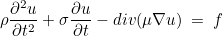
We are considering the following equation :

The physical coefficients ρ, σ and μ are specified when you write a ligne "MateriauDielec = ..." in the data file. In the case of isotropic material (μ is scalar and not a tensor), you write :
# MateriauDielec ref ISOTROPE rho mu sigma
MateriauDielec = 1 ISOTROPE 1.0 2.0 0.0
MateriauDielec = 2 ISOTROPE (1.0,0.5) (2.0,0.1) 0.0
As you can see, you can enter complex values for ρ and μ. Be careful to not introduce a space inside the complex number. The targets that compute the solution of this equation are :
- helm2D : the equation is solved in 2-D
- helm_axi : the equation is solved for an axisymmetric region, i.e. the 3-D region is assumed to be generated from the revolution of a 2-D section. The physical indexes such as rho, mu and sigma depend only on r and z. The user must provide a mesh of this 2-D section.
- helm3D : the equation is solved in 3-D
For axisymmetric computation, the solution is expanded in Fourier series
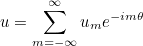
The range of modes m is specified by the keyword NumberModes. Examples of solution of Helmholtz equation are present in folders example/helm2D, example/helm3D and example/helm_axi.
Finite element formulation
When you compile helm2D or helm3D, you are solving Helmholtz equation by using one of the following classes :
- HelmholtzEquation
- HelmholtzEquationDG
For the first class, it uses the classical continuous finite element or the Symmetric Interior Penalty Galerkin (SIPG) formulation. The class HelmholtzEquationDG is implementing Local Discontinuous Galerkin (LDG) or Hybridizable Discontinuous Galerkin (HDG) formulation. The selection of the equation depends on the field TypeEquation of the data file. The following values are possible:
- HELMHOLTZ : continuous finite element method.
- HELMHOLTZ_HDG : Hybridizable Discontinuous Galerkin (HDG).
- HELMHOLTZ_SIPG : Symmetric Interior Penalty Galerkin (SIPG).
- HELMHOLTZ_DG : Local Discontinuous Galerkin (LDG).
For example the data file will contain :
TypeEquation = HELMHOLTZ
The continuous finite element method should be preferred since it is quite efficient and more functionalities are present with this formulation. For example, with the continuous finite element, the user can solve convected Helmholtz equation:

with the constraint that the flow M has a null divergence. To specify a non-null flow M, you have to write in the data file :
# first you specify that there is a flow M
AddFlowTerm = YES

# then you provide rho, mu, sigma and M (two components in 2-D)
MateriauDielec = 1 ISOTROPE 2.0 3.0 0.0  0.3 0.2
In this case, the coefficient beta is assumed to be equal to 0. If you want a coefficient beta different from 0, you should provide:
# first you specify that there is a flow M with gradient terms
AddFlowTerm = GRAD

# then you provide rho, mu, sigma and M (two components in 2-D) and beta
MateriauDielec = 1 ISOTROPE 2.0 3.0 0.0  0.3 0.2  1.0
The physical indices rho, mu, sigma, M and beta can also be provided with the keyword PhysicalMedia as follows:
PhysicalMedia = rho 1 ISOTROPE 2.0
PhysicalMedia = mu 1 ISOTROPE 1.0
PhysicalMedia = sigma 1 ISOTROPE 0.0
PhysicalMedia = M 1 ISOTROPE 0.25 0.0
PhysicalMedia = beta 1 ISOTROPE 1.0
The keyword ISOTROPE is needed, it is only meaningful for the coefficient mu. For this coefficient, you could choose ORTHOTROPE or ANISOTROPE:
# for orthotrope media, mu is diagonal (mu_xx and mu_yy in 2-D)
PhysicalMedia = mu 1 ORTHOTROPE 2.0 1.5

# for anistrope media, mu is symmetric (you give mu_xx, mu_xy and mu_yy in 2-D)
# (mu_xx, mu_xy, mu_xz, mu_yy, mu_yz and mu_zz in 3-D)
PhysicalMedia = mu 1 ANISOTROPE 2.0 0.2 1.5
For other coefficients (different from mu), a string is needed (like ISOTROPE) but it is not used. For other formulations (SIPG, HDG or LDG), the presence of the flow is not implemented. The presence of flow is implemented for axisymmetric computations (helm_axi implements only continuous finite element method), in this case it is assumed that all physical indexes (rho, mu, etc) depend only on r and z (they do not depend on θ). Moreover the flow is given in cylindrical coordinates, i.e. components Mr, Mθ and Mz are provided.
Boundary conditions
For Helmholtz equation, the following boundary conditions are implemented :
- DIRICHLET : it corresponds to the condition
where g depends on the selected source.

- NEUMANN : it corresponds to the condition
where g depends on the selected source.

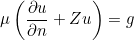
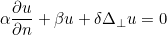
- IMPEDANCE Z : it corresponds to the condition
where g depends on the selected source. The impedance Z is given after the string IMPEDANCE, e.g.:
ConditionReference = 1 2 IMPEDANCE 2.5
sets Z to 2.5.
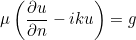
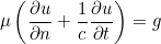
- ABSORBING : it corresponds to a first-order absorbing boundary condition
where g depends on the selected source. The wave number k is computed from physical indices rho and mu:
 Higher-order absorbing boundary conditions are available for continuous formulation.
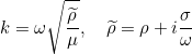
- HIGH_CONDUCTIVITY eps : it corresponds to an equivalent boundary condition
replacing an object with a high conductivity.
The parameter epsilon is given after the string HIGH_CONDUCTIVITY, for instance :

ConditionReference = 1 2 HIGH_CONDUCTIVITY 0.1
sets epsilon to 0.1.
For the high conductivity boundary condition, three orders are implemented:
where

The selection of the order is performed in the data file :
# For third-order high conductivity boundary condition :
OrderHighConductivityBoundaryCondition = 3
Absorbing boundary condition, transparent condition and PML
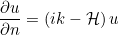
The usual absorbing boundary condition is given as

where k is the wave number. If the data file contains the following line :
ModifiedImpedance = CURVE
The absorbing boundary condition is modified as (only for continuous finite elements)
where H is the mean curvature. By default, the order of absorbing boundary condition is equal to 1. You can specify a second-order absorbing boundary condition by writing :
OrderAbsorbingBoundaryCondition = 2
ModifiedImpedance = CURVE
In that case, the following boundary condition is applied :
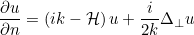
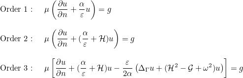
This absorbing boundary condition involves the Laplace Beltrami operator. This condition is not implemented for discontinuous formulation (LDG or HDG). More accurate absorbing boundary conditions are implemented for continuous finite elements. They are all second-order absorbing boundary condition, even though they are listed with higher orders. If you write
OrderAbsorbingBoundaryCondition = 3
ModifiedImpedance = CURVE
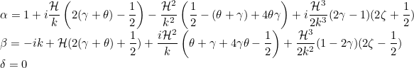
The following absorbing boundary condition is applied
with the coefficients:
If you write
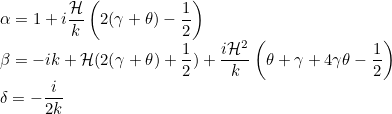
OrderAbsorbingBoundaryCondition = 4
ModifiedImpedance = CURVE
The coefficients are given as
If you write
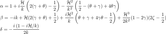
OrderAbsorbingBoundaryCondition = 5
ModifiedImpedance = CURVE
The coefficients are given as
The default values of parameters are equal to:
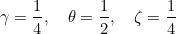
If you want to specify different values, you can write
# order PARAMETERS gamma theta zeta
OrderAbsorbingBoundaryCondition = 5 PARAMETERS 0.2 0.4 0.2
ModifiedImpedance = CURVE
A transparent condition has been implemented based on an integral representation. It needs the definition of a intermediary boundary between the extern boundary and the scattered objects. It is assumed that the medium between this intermediary boundary and the extern boundary is homogeneous such that the integral representation is correct. On the extern boundary, the user must specify a first-order absorbing boundary condition (without curvature terms). The intermediary boundary is given through a body number. For instance, if the body 1 comprises edges (faces in 3-D) of reference 2, 4 et 7, the data file must contain
TypeBody = 2 1
TypeBody = 4 1
TypeBody = 7 1
Then, to activate the transparent condition, the data file must contain the two lines :
# YES body_number order
TransparencyCondition = YES 1 AUTO
# GMRES nb_iter_max stopping_criterion restart
ParamResolutionTransparency = GMRES 100 1e-8 10
Perfectly Matched Layers (PML) can be added in the computational domain, they are usually more efficient than absorbing boundary conditions since you can adjust the reflection coefficient as small as you want. You can look at the documentation of AddPML and DampingPML to know how to add them.
Definition of source
As introduced below, f denotes a volumetric source (right hand side of the equation) while g denotes a surfacic source (right hand side of boundary conditions). For Helmholtz equation you can choose between the following sources
- SRC_VOLUME / SRC_SURFACE / SRC_MODE: f and g are specified for each reference
- SRC_DIRAC : f is a Dirac (all g are null)
- SRC_USER : f and g are given in UserSource.cxx
- SRC_TOTAL_FIELD : the total field is computed
- SRC_DIFFRACTED_FIELD : the diffracted field is computed
When you write SRC_VOLUME, by default the support of f contains all the references of the mesh. For example if you have written:
# TypeSource = SRC_VOLUME GAUSSIAN x0 y0 r0 r1
TypeSource = SRC_VOLUME GAUSSIAN 0 0 1.0 2.0
f will be a gaussian :
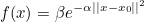
with the following parameters
x0 is the center of the gaussian (the two first parameters), r0 the radius of the gaussian. The parameter r1 is optional and is used to truncate the gaussian, we set :
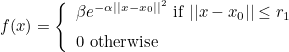
If not specified, r1 is equal to r0. You can choose also uniform function (instead of gaussian) :
# TypeSource = SRC_VOLUME UNIFORM
TypeSource = SRC_VOLUME UNIFORM
In that case, f is equal to 1 in all the space. You can specify a support for f, by giving the reference (corresponding to Physical Surface in gmsh) where it is non-null. For example, if you write:
# TypeSource = SRC_VOLUME ref UNIFORM
TypeSource = SRC_VOLUME 2 UNIFORM
f will be equal to 1 on elements of reference 2, and 0 otherwise. You can also provide the source f on quadrature points with keyword VARIABLE_BINARY:
# TypeSource = SRC_VOLUME ref VARIABLE_BINARY file
TypeSource = SRC_VOLUME 2 VARIABLE_BINARY value.dat

# if you use GRADIENT BINARY, it corresponds to the integral against gradient of basis functions
TypeSource = SRC_VOLUME 2 GRADIENT_BINARY value.dat
A detailed description of this functionality is given in the documentation of TypeSource keyword.
Surface sources (functions g) are always affected to a given reference :
# TypeSource = SRC_SURFACE 2 GAUSSIAN x0 y0 r0 r1 Polarization
TypeSource = SRC_SURFACE 2 GAUSSIAN 0 0 1.0 2.0 Polarization 20.0
Polarization is used to specify an amplitude different from one for this function g. The function g can be either uniform (the constant is set with the Polarization) either gaussian or a plane wave . A last option is a variable function known on points. In this case, you must provide the list of 2-D (or 3-D for 3-D simulation) points where the function g is known and the associated value. An example is provided in the documentation of TypeSource. For Helmholtz equation, the values must be complex (as in the example). For a variable function, the number of points where g is known must be larger than the number of quadrature points on each edge/face of the mesh. If it is not the case, an error message will be displayed.
SRC_MODE is used to set g as a Laplacian mode over the given section with the following syntax :
# TypeSource = SRC_MODE ref MODE shift nb_modes nb_modes_combine n0 coef0 n1 coef1 ... boundary_condition
TypeSource = SRC_MODE 1 MODE 0.1 2 1 1 1.0 DIRICHLET
shift is the shift used to find eigenvalues (in 3-D), nb_modes is the number of eigenvalues to compute (closest to shift), nb_modes_combine is the number of eigenvectors that will be combined to obtain the function g, n0, coef0, n1, coef1... are the different mode numbers and coefficients used to compute g (which is obtained as a linear combination of eigenmodes) . Finally, you must specify which boundary condition is set on the boundary of the section (DIRICHLET or NEUMANN).
If you select, SRC_TOTAL_FIELD or SRC_DIFFRACTED_FIELD, the solution is sought in the form

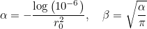
The incident field can be chosen between a plane wave, Hankel wave, a gaussian beam or a layered plane wave (expressions are detailed in the documentation of TypeSource). In this case, the incident field is mandatory (keyword IncidentAngle). By default, the origin of the phase is equal to (0, 0), you can modify it with the keyword OriginePhase. For a plane wave for example, you have the following the following expression:
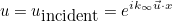
The direction of the wave vector (denoted
 ) is given through the keyword IncidentAngle. The wave number at infinity is given as:
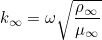
The value of ρ and μ at infinity are by default set to 1. If you have different values, you need to enter a line with the keyword ReferenceInfinity:
# ReferenceInfinity = ref
ReferenceInfinity = 1
Here the reference number is the physical reference associated with elements (triangles/quadrilaterals in 2-D). For a layered plane wave, you need to provide the value of ρ and μ for internal layers only since we assume that for the two external layers (z < z0 and z > zN) ρ and μ are the indices at the infinity.
# for one internal layer, you put LAYERED_PLANE_WAVE 1 z0 rho0 mu0 z1
# where z0 and z1 are the boundaries of the internal layer, and rho0 mu0 the values of rho mu inside this layer
TypeSource = SRC_DIFFRACTED_FIELD LAYERED_PLANE_WAVE 1 -0.8 2.0 3.0 1.2
When you specify SRC_TOTAL_FIELD, the total field is computed. As a result, there will source terms because of absorbing boundary conditions or PMLs. For absorbing boundary conditions, only first-order absorbing boundary condition should work correctly with SRC_TOTAL_FIELD. For higher absorbing boundary conditions, you will have to use SRC_DIFFRACTED_FIELD. When this source is selected, the diffracted field is computed, source terms appear on boundary conditions (such as Neumann or impedance conditions) and on dielectric media. SRC_DIFFRACTED_FIELD is not implemented on other models (such as transmission conditions or thin slot model).
Other models
Basic thin slot model (see Tordeux thesis) is implemented in 2-D only. It is based either on a 1-D discretization of the slot or a DtN operator. An example is given in example/helm2D/modele_fente.ini. You have to add in the data file :
# AddSlot = x0 y0 x1 y1 epsilon nb_points
AddSlot = -0.5 0 0.5 0  0.01 10

# ModelSlot = model (either 1D_MESH or DTN)
ModelSlot = 1D_MESH
Laplace equation
For stationary problems, we have defined a Poisson's equation :

LaplaceEquation and LaplaceEquationDG are implementing this last equation in real numbers (rho and mu are real as well as the solution). The file to compile is located in src/Program/Advanced/laplace.cc and can be compiled with target laplace:
make laplace
If the selected finite element is a triangle/quadrilateral (like TRIANGLE_LOBATTO), the computation will be performed in 2-D, otherwise it will be performed in 3-D. You can choose between the following equations:
- LAPLACE : continuous finite element method.
- LAPLACE_HDG : Hybridizable Discontinuous Galerkin (HDG).
- LAPLACE_SIPG : Symmetric Interior Penalty Galerkin (SIPG).
- LAPLACE_DG : Local Discontinuous Galerkin (LDG).
The boundary conditions and indices are similar to those defined for Helmholtz equation. Examples of solutions of Laplace equation are present in folders example/laplace.
Acoustics equation (wave equation)
The stationary problem defined by LaplaceEquation or LaplaceEquationDG is used for the solution of the following wave equation
If you are using a time-scheme for first-order problems (in time), you are actually solving this system :
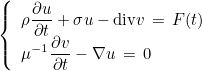
where F is the primitive of f. PML layers are only implemented within this first-order system. AcousticEquation is the class for the solution of acoustics with continuous finite elements, whereas AcousticEquationDG is used for discontinuous Galerkin method. The targets are the following ones:
- acous2D : the equation is solved in 2-D
- acous_axi : the equation is solved for an axisymmetric region, i.e. the 3-D region is assumed to be generated from the revolution of a 2-D section. The physical indexes such as rho, mu and sigma depend only on r and z. The user must provide a mesh of this 2-D section.
- acous3D : the equation is solved in 3-D
Examples of solutions of wave equation are present in folders example/acous2D, example/acous3D and example/acous_axi. You can choose between the following equations
- ACOUSTIC : continuous finite element method.
- ACOUSTIC_HDG : Hybridizable Discontinuous Galerkin (HDG).
- ACOUSTIC_SIPG : Symmetric Interior Penalty Galerkin (SIPG).
- ACOUSTIC_DG : Local Discontinuous Galerkin (LDG).
The implementation of ACOUSTIC_SIPG is quite experimental, and can be used only for second-order time schemes (such as RUNGE_KUTTA_NYSTROM) without any damping term (no absorbing condition, σ is equal to 0). The physical indices rho, mu and sigma are given in the datafile as explained in the case of Helmholtz equation. PML layers are available for ACOUSTIC or ACOUSTIC_DG.
Boundary conditions
The following boundary conditions are available:
- DIRICHLET : it corresponds to the condition
where g depends on the selected source.

- NEUMANN : it corresponds to the condition
where g depends on the selected source.

- ABSORBING : it corresponds to a first-order absorbing boundary condition
where g depends on the selected source. The velocity c is computed from physical indices rho and mu:
 Higher-order absorbing boundary conditions are not available.
Sources
You can define two types of sources
A source with separation of variables. Each f (volume source) and g (surface source) are equal to

The space sources (here f(x) or g(x)) are given with lines TypeSource:
TypeSource = SRC_VOLUME 1 GAUSSIAN ...
TypeSource = SRC_SURFACE 2 UNIFORM ...
TypeSource = SRC_SURFACE 2 GAUSSIAN ...
whereas the temporal source (here h(t)) is given with a line TemporalSource:
// see the documentation for a list a available time sources
TemporalSource = RICKER
Usually, the temporal source uses also the field Frequency to retrieve the central frequency of the pulse.
A plane wave source, the source comes from an incident plane wave. The datafile should contain a line
# computation of the scattered field
# TypeSource = SRC_DIFFRACTED_FIELD offset
TypeSource = SRC_DIFFRACTED_FIELD AUTO
if the diffracted field is computed, or a line
# computation of the total field
# TypeSource = SRC_TOTAL_FIELD offset
TypeSource = SRC_TOTAL_FIELD AUTO
if the total field is computed. The incident field is given as
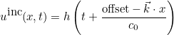
where h is the temporal source (given with a line TemporalSource), c0 the velocity at infinity (different from 1 if the field ReferenceInfinity has been provided),
 the wave vector, and offset computed as
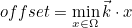
if you have specified AUTO in the datafile (for the TypeSource line). The wave vector k has a norm equal to 1 here, and is provided by the keyword IncidentAngle. If the diffracted field is computed (SRC_DIFFRACTED_FIELD), a source term appears for Dirichlet and Neumann boundaries. In theory, a source term should appear for dielectric objects, but this source term is not implemented for acoustic wave equation (contrary to Helmholtz), so the solution should be false in this case. If the total field is computed (SRC_TOTAL_FIELD), a source appears for absorbing boundaries. In theory, a source term should appear in PML layers, but it is not implemented (contrary to Helmholtz), so the solution should be false in this case.
Solution in 1-D or with radial symmetry
Helmholtz equation and Laplace equation are also implemented in 1-D with a specific implementation (outside of the class VarHarmonic) in the files Helmholtz1D.hxx and Helmholtz1D.cxx. The associated equations are HelmholtzEquation1D and LaplaceEquation1D. The leaf class EllipticProblem for these two equations derive from the base class VarHelmholtz_1D.
Methods for class VarHelmholtz_1D
| SetInputData | modifies parameters of the problem with a line of the data file |
| GetMiomega | returns -i ω for Helmholtz equation, 1 for Laplace equation |
| GetIkwave | returns i k(ω) for Helmholtz equation, 1 for Laplace equation |
| SetOmega | changes the value of the pulsation ω |
| ComputeMassMatrix | computes intermediary arrays needed for the computation of the finite element matrix |
| GetMassMatrix | fills the mass matrix (if lumped) |
| GetDampingMatrix | fills the damping matrix (if lumped) |
| GetStiffnessMatrix | returns the local stiffness matrix |
| GetGradientMatrix | returns the local gradient matrix |
| GetLocalMassMatrix | returns the local mass matrix |
| InitIndices | sets the number of physical domains |
| SetIndices | sets the indices rho, sigma, mu for a physical domain |
| GetVelocityOfMedia | returns the velocity of a physical domain |
| EvaluateFuncionTauPML | computes the damping function τ inside the PML |
| GetDampingTauPML | computes the damping term ζ inside the PML |
| ComputeMeshAndFiniteElement | computes the mesh and finite element |
| AddDomains | assembles a vector (in case of parallel computations) |
| GetXmin | returns the left extremity of the computational domain |
| GetXmax | returns the right extremity of the computational domain |
| GetNbDof | returns the number of degrees of freedom of the problem |
| GetFaceBasis | returns the finite element class of a given order |
| GetLeafClass | returns the leaf class EllipticProblem |
| RunAll | completes a global simulation |
| AddVolumetricSource | adds volumetric integrals to a vector |
| AddSurfacicSource | adds surface terms to a vector |
| AddVolumetricProjection | adds projection of a function on degrees of freedom |
| ComputeRightHandSide | computes the right hand side |
| TreatDirichletCondition | treats Dirichlet condition if present |
| AddBoundaryTerms | adds terms due to the boundary condition in the finite element matrix |
| AddMatrixFEM | adds terms due to volume integrals in the finite element matrix |
| WriteDatas | writes the solution in output files |
| ComputeInterpolationU | computes the interpolation of the solution on a predefined grid |
| GetInterpolate | computes the interpolation of the solution on a single point |
Helmholtz equation can be solved in spherical geometries (this case is referred as a solution with radial symmetry, since the geometry depends only on r), the implementation of this special case is done in the files HelmholtzRadial.hxx and HelmholtzRadial.cxx. The associated equation is HelmholtzEquationRadial. The leaf class EllipticProblem for this equation derive from the base class VarHelmholtz_Radial.
Methods for class VarHelmholtz_Radial
| GetLmax | returns the maximum
 (maximal order of the spherical harmonics)
 |
| SetInputData | modifies parameters of the problem with a line of the data file |
| ConstructAll | constructs all the arrays needed before calling PerformFactorizationStep |
| ComputeVarGrid | computes the interpolation grid (points of the grid are localized in the mesh) |
| PerformFactorizationStep | computes and factorizes the finite
element matrix for a given

|
| ComputeSolution | solves the linear system satisfied by the solution |
| ComputeIncidentField | computes the decomposition of the incident plane wave in spherical harmonics |
| ComputeRightHandSide | computes the right hand sides of the linear systems satisfied by the solutions |
| ComputeRhsDiffractedField | computes the right hand sides in the case where the diffracted field is searched |
| ComputeRhsTotalField | computes the right hand sides in the case where the total field is searched |
| WriteDatas | writes the solution in output files |
Solution in axisymmetric domains
Helmholtz equation can be solved in cylindrical coordinates (r, θ, z) where the geometry depends only on r and z. In that case, only the 2-D section (r, z) of the generating surface must be meshed. The source may depend on θ and is expressed as a Fourier serie in θ. Each component of the Fourier serie solves an independent equation, the implementation of these equations is performed in the files AxiSymHelmholtz.hxx, AxiSymHelmholtzInline.cxx and AxiSymHelmholtz.cxx. The class EllipticProblem for the equation HelmholtzEquationAxi derives from the class VarHelmholtz_Axi.
Methods for class VarHelmholtz_Axi
| SetInputData | modifies parameters of the problem with a line of the data file |
| SwapFiniteElement | switches to the appropriate finite element class for the current element |
| GetNbModesSource | returns the number of Fourier modes in the source |
| PushBackMode | adds a mode to be solved in the list of modes |
| InitIndices | sets the number of physical domains |
| GetVaryingMedia | retrieves all the varying scalar fields fro physical indices |
| SetIndices | sets the physical indices
 for a given domain
|
| GetNbPhysicalIndices | returns the number of physical domains |
| IsVaryingMedia | returns true if the physical domain i contains a varying index |
| GetVelocityOfMedia | returns the velocity of the physical domain i |
| GetVelocityOfInfinity | returns the velocity at infinity |
| IsSymmetricProblem | returns true if the finite element matrix is symmetric |
| UseNumericalIntegration | returns true if numerical integration should be performed on element i |
| IsElementNearAxis | returns true if the element i contains a point on the axis |
| GetWaveVector | returns the wave vector |
| GetPhaseOrigin | returns the origin of phase for the plane wave |
| GetFourierMode | returns
 or
or

|
| InitCyclicDomain | inits symmetries of the simulation |
| FindELementsInsidePML | finds all the elements that are inside the PML |
| SetPhysicalIndexAtInfinity | not documented |
| GetCoefficientPML | computes some coefficients in the PML |
| GetTampingTauPML | computes the coefficients
 in the PML
|
| ConstructAll | computes all the arrays needed before computing the finite element matrix |
| WriteAllIndices | writes the physical indexes in output files |
| PerformAdimensionalization | performs an adimensionalization on the physical indexes and unknown |
| PutAdditionalDofsAndOtherInitializations | complete other initializations |
| AllocateMassMatrices | allocates the arrays needed to store geometric quantities |
| ComputeLocalMassMatrix | computes geometric quantities for an element of the mesh |
| GetNbRightHandSide | returns the number of right hand sides |
| ComputeRightHandSide | computes the right hand side |
| AddDiracSource | adds a Dirac to the right hand side |
| ModifyOutputUnknown | modifies the solution u before writing it to the output files |
| ModifyOutputGradient | modifies the gradient of the solution u before writing it to the output files |
| WriteDatas | writes the solution on output files |
Helmholtz equation in 2-D and 3-D
The implementation of Helmholtz equation (and Laplace equation) in 2-D and 3-D is performed in the files VarHelmholtz.cxx and VarLaplace.cxx. The files DefineSourceHelmholtz.cxx and LaplacianModalSource.cxx implements the different sources (diffracted field, total field, mode on a section) for Helmholtz equation. In the file HelmholtzHdiv.cxx, a H(div) formulation is implemented although this formulation is not efficient in practice. The different impedance conditions (including absorbing boundary conditions) for Helmholtz equations are present in the file ImpedanceHelmholtz.cxx. The models for thin slots are implemented in 2-D in the file ThinSlotHelmholtzModel.cxx. Transmission conditions are proposed (they replace a thin layer) in the file TransmissionModelHelmholtz.cxx.
Methods for class VarHelmholtz_Base
| SetInputData | modifies parameters of the problem with a line of the data file |
| SetFirstOrderFormulation | sets a first-order formulation instead of second-order |
| InitIndices | sets the number of physical domains |
| GetNbPhysicalIndices | returns the number of physical domains |
| SetIndices | sets the physical indices
 for a given domain
|
| CopyIndices | copies the physical indices of another Helmholtz problem |
| CopyIndicesMaxwell | copies the physical indices of Maxwell's problem |
| IsVaryingMedia | returns true if the physical domain i contains a varying index |
| GetVaryingIndices | retrieves all the varying fields from physical indexes |
| GetVelocityOfMedia | returns the velocity of the physical domain i |
| GetVelocityOfInfinity | returns the velocity at infinity |
| GetCoefficientPenaltyStiffness | returns the coefficient associated with a physical domain for penalty terms |
| FinalizeComputationVaryingIndices | finalizes the computation of physical indices on quadrature points |
| GetPhysicalCoefPML | fills coefficients
 inside the PMLs.
|
| IsSymmetricProblem | returns true if the finite element matrix is symmetric |
| HasMatrixComplexCoefficients | returns true if the finite element matrix will contain complex non-zero entries |
| GetMuIntegrationByParts | returns the physical index involved in the boundary term of integration by parts |
| ModifyOutputUnknown | modifies the solution u before writing it to the output files |
| GetEnHnQuadrature | forms u and du/dn from u and gradient of u |
| GetEnHn | forms u and du/dn from u and gradient of u |
| AllocateMassMatrices | allocates arrays needed to store geometric quantities |
| ComputeNumberOfDofs | computes the number of degrees of freedom of the problem |
| PutOtherGlobalDofs | adds other degrees of freedom |
| TreatDirichletCondition | treats Dirichlet condition |
| PutAdditionalDofsAndOtherInitializations | performs other initializations before computing geometric quantities |